This page contains the notes for the first part of R Workshop Module 5: Statistical modeling with R, which is part of the R Workshop series prepared by ICJIA Research Analyst Bobae Kang to enable and encourage ICJIA researchers to take advantage of R, a statistical programming language that is one of the most powerful modern research tools.

Statistical modleing with R (1): Basics of statistical modeling

R is first designed as a programming language and an environment for statistics and data analysis. Accordingly, R provides as part of its base packages a host of handy tools for conducting statistical analysis. This part introduces the basics of descriptive and inferential statistics in R and touches on fitting linear and generalized linear models.

Basic Descriptive Statistics

Source: Vadlo.com

Quick summary stats

summary(data)

The Base R summary() function is a quick way to get descriptive statistics on each columan of a tabular data object.

For numerical columns, we get the minimum, 1st quartile, median, mean, 3rd quartie and maximum values, as well as the count of missing value (NA).

For categorical variables (e.g. factor), we can the count for each level as well as the missing value (NA).

summary() is also used to get the “summary” of a fitted model object (e.g. lm) as well, as we will see shortly.

Example

Let’s take a look at summary of the ispcrime dataset.

summary(ispcrime)

##       year            county     violentCrime       murder       
##  Min.   :2011   Adams    :  5   Min.   :    0   Min.   :  0.000  
##  1st Qu.:2012   Alexander:  5   1st Qu.:   19   1st Qu.:  0.000  
##  Median :2013   Bond     :  5   Median :   42   Median :  0.000  
##  Mean   :2013   Boone    :  5   Mean   :  501   Mean   :  7.026  
##  3rd Qu.:2014   Brown    :  5   3rd Qu.:  133   3rd Qu.:  1.000  
##  Max.   :2015   Bureau   :  5   Max.   :33348   Max.   :566.000  
##                 (Other)  :480   NA's   :7       NA's   :7        
##       rape            robbery          aggAssault      propertyCrime   
##  Min.   :   0.00   Min.   :    0.0   Min.   :    0.0   Min.   :     0  
##  1st Qu.:   1.00   1st Qu.:    0.0   1st Qu.:   15.0   1st Qu.:   133  
##  Median :   6.00   Median :    2.0   Median :   33.0   Median :   349  
##  Mean   :  41.29   Mean   :  172.3   Mean   :  280.4   Mean   :  2913  
##  3rd Qu.:  22.00   3rd Qu.:   13.0   3rd Qu.:  102.0   3rd Qu.:  1190  
##  Max.   :1986.00   Max.   :16095.0   Max.   :15129.0   Max.   :178902  
##  NA's   :7         NA's   :7         NA's   :7         NA's   :7       
##     burglary         larcenyTft           MVTft             arson        
##  Min.   :    0.0   Min.   :     0.0   Min.   :    0.0   Min.   :   0.00  
##  1st Qu.:   35.5   1st Qu.:    85.5   1st Qu.:    3.0   1st Qu.:   1.00  
##  Median :   79.0   Median :   258.0   Median :   10.0   Median :   2.00  
##  Mean   :  589.3   Mean   :  2084.9   Mean   :  215.2   Mean   :  23.45  
##  3rd Qu.:  268.0   3rd Qu.:   852.0   3rd Qu.:   30.0   3rd Qu.:   8.50  
##  Max.   :38485.0   Max.   :116145.0   Max.   :22879.0   Max.   :1418.00  
##  NA's   :7         NA's   :7          NA's   :7         NA's   :7

Numerical variables

A distribution of numerical values can be described using statistics on the following characteristics:

Central tendency
Variability
Shape
Outliers

In the following, we will briefly discuss what each of these characteristics means and how we can get relevant statistics in R.

Central tendency

In statistics, central tendency is concerned with the “center” of a distribution. The following three are the common measures of central tendency:

“mean” for the arithmetic mean
“median” for the 50th percentile
“mode” for the most frequent value

R has built-in functions for the first two: mean() and median(). Unfortunately, there is no native R function for mode. However, it is possible to create a custom function using the definition, i.e. the most frequnt value. Also, check out the modeest package that offers mode estimators.

Let us try using mean() and median() for the violentCrime column. And the result is …

mean(ispcrime$violentCrime)

## [1] NA

median(ispcrime$violentCrime)

## [1] NA

… wait, what? We get NA for both values.

This is because NA in R is a “contagious” value, making any operation with missing values return NA. To remedy this, we can use the na.rm argument, which takes a boolean input to control weather whether NA values are removed/excluded in calculation. The default is na.rm = FALSE

We try again with na.rm = TRUE:

mean(ispcrime$violentCrime, na.rm = TRUE)

## [1] 500.9702

median(ispcrime$violentCrime, na.rm = TRUE)

## [1] 42

Variability

Variability (or dispersion) in statistics is concerned with the extent to which a distribution is spreaded out.

There exist various measures for variability and R has built-in functions for many of them:

range: min(), max(), range()
percentiles: fivenum(), IQR(), quantile()
variance: var(), sd()

Range

Range is the interval between the minium nad maximum values. R offers min for getting the minimum value, max() for the maximum value, and range() for the range. Each of functions has the na.rm argument, so make sure change its input as needed.

min(ispcrime$violentCrime, na.rm = TRUE)

## [1] 0

max(ispcrime$violentCrime, na.rm = TRUE)

## [1] 33348

range(ispcrime$violentCrime, na.rm = TRUE)

## [1]     0 33348

Percentiles

R has a few useful functions to inspect the distribution of numerical data in terms of percentiles.

The fivenum() function returns what is called Tukey’s five number summary (minumum, 1st quartile, median, 3rd qurtile, maximum) for the input data. IQR() returns the inter-quartile range, which is the difference between the 1st quartile (25%) and 3rd quartile (75%).

The following shows the outputs of these functions using violentCrime as the input:

fivenum(ispcrime$violentCrime, na.rm = TRUE)

## [1]     0    19    42   133 33348

IQR(ispcrime$violentCrime, na.rm = TRUE)

## [1] 114

quntile() is a somewhat more flexible function. The default setting output of quantile() is equal to fivenum() output. However, quantile() can use probs arugment to get more flexible output.

# default: equal to fivenum()
quantile(ispcrime$violentCrime, probs = seq(0, 1, 0.25), na.rm = TRUE)

##    0%   25%   50%   75%  100% 
##     0    19    42   133 33348

quantile(ispcrime$violentCrime, probs = seq(0, 1, 0.1), na.rm = TRUE)

##      0%     10%     20%     30%     40%     50%     60%     70%     80% 
##     0.0     5.0    13.0    24.0    32.0    42.0    57.0    90.0   246.2 
##     90%    100% 
##   668.4 33348.0

Variance

The R function for variance is var(), which returns the sample variance of the given data: \[s^2 = (\sum{x - \bar{x}}^2)/(n-1)\]

var(ispcrime$violentCrime, na.rm = TRUE)

## [1] 9463013

Similarly, sd() returns the standard deviation of the given data: \[s = \sqrt{(\sum{x - \bar{x}}^2)/(n-1)}\]

sd(ispcrime$violentCrime, na.rm = TRUE)

## [1] 3076.201

Note that var() returns a covariance matrix when multiple variables are given as its input. In such cases, another function named cov() can be used instead for clarity; however, cov() has no na.rm argument to handle missing values.

variables <- ispcrime %>% select(violentCrime, propertyCrime)
var(variables, na.rm = TRUE)

##               violentCrime propertyCrime
## violentCrime       9463013      46803865
## propertyCrime     46803865     234761775

Shape

The skewness and kurtosis (fatness/thinness) of a distribution are called the “shape” of the distribution.

While base R has no functions to get these statistics (which are rarely used for common descriptive statistics anyway), the moments package offers the following functions to meaasure the shape of a distribution:

skewness()
kurtosis()

See moments package’s reference manual to find out more.

Outliers

Outliers are observations or data points that are far from most other observations and disproportinately affect key summary statistics

The outliers package offers useful functions to detect and measure outliers in data. See outliers package’s reference manual to learn more.

Categorical variables

Inspecting the distribution of a categorical variable requires a different set of tools. Frequency table is one of the most common ways to summarize the distribution of a catagorical variable.

In R, frequency tables can be made using table functions. We will take a look at the following:

table() for generating frequency tables
prop.table() for tables of proportions
xtabs() for creating frequency tables using formula
ftable() for creating “flat” contingency tables

Table functions

table(...)
prop.table(x, margin = NULL)
ftable(x)
xtabs(formula, data, ...)

table() takes one or more data vectors of same length. Each input data can be named like in the case of creating a list or a data.frame object. We can use as.data.frame() to turn a table into a data frame.

Both prop.table() and ftable() takes a table object. prop.table() returns a table in terms of proportion, where \(0 \leq p \leq 1\) for each value. ftable() returns a flat contingency table. We will shorty see what this means with an example below.

Finally, xtabs use formula to generate a frequency table. If a data frame is provided as the data input, its column names can be used directly in formula.

`table()` example

First, let us create a data to use for creating tables:

my_data <- ispcrime %>%
  left_join(regions) %>%
  select(
    region,
    viol = violentCrime,
    prop = propertyCrime
  ) %>%
  mutate(
    high_viol = ifelse(viol > mean(viol, na.rm = TRUE), 1, 0),
    high_prop = ifelse(prop > mean(prop, na.rm = TRUE), 1, 0)
  )

## Joining, by = "county"

Now, we create a table object with two dimensions: region for regions in the state, and hviol for the greater-than-average violent crime count.

my_tbl <- table(
  region = my_data$region,
  hviol = my_data$high_viol
)

Now we print the table.

my_tbl

##           hviol
## region       0   1
##   Central  206  24
##   Cook       0   5
##   Northern  60  25
##   Southern 175   8

We can turn it into a data.frame, which can be more easily manipulated.

as.data.frame(my_tbl)

##     region hviol Freq
## 1  Central     0  206
## 2     Cook     0    0
## 3 Northern     0   60
## 4 Southern     0  175
## 5  Central     1   24
## 6     Cook     1    5
## 7 Northern     1   25
## 8 Southern     1    8

`prop.table()` example

prop.table() has a margin argument to control how to generate margin for. magin takes an index, or vector of indices as an input. Take a look at the following examples to see how margin argument works:

prop.table(my_tbl, 1) # each row adds up to 1

##           hviol
## region              0          1
##   Central  0.89565217 0.10434783
##   Cook     0.00000000 1.00000000
##   Northern 0.70588235 0.29411765
##   Southern 0.95628415 0.04371585

prop.table(my_tbl, 2) # each column adds up to 1

##           hviol
## region              0          1
##   Central  0.46712018 0.38709677
##   Cook     0.00000000 0.08064516
##   Northern 0.13605442 0.40322581
##   Southern 0.39682540 0.12903226

If margin input is , each cell is x/sum(x).

`ftable()` example

To better illustrate what ftable() does, we first create a table with three dimensions. This is becuase using ftable() for a table of 2 dimensions or less makes little difference.

my_tbl2 <- table(
  region = my_data$region,
  hviol = my_data$high_viol,
  hprop = my_data$high_prop
)

Now, we first see the ftable() output.

# with ftable
ftable(my_tbl2)

##                hprop   0   1
## region   hviol              
## Central  0           197   9
##          1             1  23
## Cook     0             0   0
##          1             0   5
## Northern 0            55   5
##          1             0  25
## Southern 0           173   2
##          1             0   8

Then compare it to the default printing otuput.

# without ftable
my_tbl2

## , , hprop = 0
## 
##           hviol
## region       0   1
##   Central  197   1
##   Cook       0   0
##   Northern  55   0
##   Southern 173   0
## 
## , , hprop = 1
## 
##           hviol
## region       0   1
##   Central    9  23
##   Cook       0   5
##   Northern   5  25
##   Southern   2   8

`xtabs()` example

xtabs() creates an xtabs object, which is built on top of table. Creating one-dimensional table with xtabs() looks like the following:

# one-dimension
xtabs(~ region, my_data)

## region
##  Central     Cook Northern Southern 
##      230        5       85      190

Adding more dimensions can be done usign the + operator in the formula:

# two-dimension
xtabs(~ region + high_viol, my_data)

##           high_viol
## region       0   1
##   Central  206  24
##   Cook       0   5
##   Northern  60  25
##   Southern 175   8

Basic Inferential Statistics

Source: Vadlo.com

Student’s t-test

t.test(x, y = NULL, alternative = c("two.sided", "less", "greater"),
       mu = 0, conf.level = 0.95, ...)
t.test(formula, data, subset, na.action, ...)

R offers the t.test() function to conduct Student’s t-test. x and y are numeric vectors of data values.

If only x is given, one sample t-test is conducted and the mean of x is compared agianst the mu value with the default of 0. If both x and y are provided, two sample t-test is conducted.

The test null hypothesis is no difference in the sample means, assuming that each sample comes from a normal distribution.

alternative defines the alternative hypothesis, which can take the value of “two.sided” (default), “less”, or “greater”.

Two sample t-test can also be conducted by using formula (y ~ x) with data input.

Example

Let’s take a look at an example of using t.test(). First we prepae x and y to use.

ispcrime2 <- left_join(ispcrime, regions)

## Joining, by = "county"

viol_crime_north <- (filter(ispcrime2, region == "Northern"))$violentCrime
viol_crime_south <- (filter(ispcrime2, region == "Southern"))$violentCrime

Now we conduct two sample t-test using viol_crime_north and viol_crime_south with the default “two.sided” alternative hypothesis:

t.test(viol_crime_north, viol_crime_south)

## 
##  Welch Two Sample t-test
## 
## data:  viol_crime_north and viol_crime_south
## t = 4.4064, df = 105.49, p-value = 2.534e-05
## alternative hypothesis: true difference in means is not equal to 0
## 95 percent confidence interval:
##  176.7132 465.8398
## sample estimates:
## mean of x mean of y 
##  438.2000  116.9235

Wilcoxon tests

wilcox.test(x, y = NULL, alternative = c("two.sided", "less", "greater"),
            mu = 0, conf.level = 0.95, ...)
wilcox.test(formula, data, subset, na.action, ...)

R offers wilcox.test() for Wilcoxon tests. It is often considered a nonparametric counterpart of the t-test, and can be performed using either one sample or two samples. Unliked in Student’s t-test, Wilcoxon test does not assume normality.

One sample Wilcoxon test (i.e. rank-sum test) is conducted with only x input is provided.

Two sample Wilcoxon test (singed-rank test) can be conducted by either supplying x and y inputs or using formula (y ~ x) with data input.

Analysis of Variance

aov(formula, data, qr = TRUE, ...)

aov() is the built-in R function to perform analysis of variance (ANOVA) to analyze the differences among group means.

Here we use formula in the following format: value ~ subgroup. data is a data.frame with both value and subgroup as its columns.

summary() has a method for aov class that returns a refined print result. Also, model.tables() has a method for aov class for reporting table of means or table of effects.

Example

This example is to illustrate different printing methods for the ANOVA model results. We first fit the model, using violentCrime as the value column and region as the subgroup column.

aov_by_region <- aov(formula = violentCrime ~ region, data = ispcrime2)

Here is the default printing output:

print(aov_by_region)

## Call:
##    aov(formula = violentCrime ~ region, data = ispcrime2)
## 
## Terms:
##                     region  Residuals
## Sum of Squares  4657351567   93080910
## Deg. of Freedom          3        499
## 
## Residual standard error: 431.8969
## Estimated effects may be unbalanced
## 7 observations deleted due to missingness

And here is using summary(), of which the ouput includes the F statistic and the relevant p-value:

summary(aov_by_region)

##              Df    Sum Sq   Mean Sq F value Pr(>F)    
## region        3 4.657e+09 1.552e+09    8323 <2e-16 ***
## Residuals   499 9.308e+07 1.865e+05                   
## ---
## Signif. codes:  0 '***' 0.001 '**' 0.01 '*' 0.05 '.' 0.1 ' ' 1
## 7 observations deleted due to missingness

Finally, using model.tables with different type input, we get the tables of means and effects:

model.tables(aov_by_region, type = "means")

## Tables of means
## Grand mean
##          
## 500.9702 
## 
##  region 
##     Central  Cook Northern Southern
##         170 30848    438.2    116.9
## rep     230     5     85.0    183.0

model.tables(aov_by_region, type = "effects")

## Tables of effects
## 
##  region 
##     Central  Cook Northern Southern
##        -331 30347   -62.77     -384
## rep     230     5    85.00      183

Other statistical tests

The following is a list of other statistical tests with built-in R fuctions:

# Test of equal proprtions
prop.test(x, n, p, ...)

# Chi-square test of indepndence/goodness-of-fit
chisq.test(x, y = NULL, ...)

# Shapiro-Wilk test of normality
shapiro.test(x)

# One- or two-sample Kolmogorov-Smirnov test
ks.test(x, y, ..., alternative = "two.sided", exact = NULL)

# F-test to compare variances
var.test(x, y, ratio = 1, alternative = "two.sided",
         conf.level = 0.95, ...)
var.test(formula, data, subset, na.action, ...)

# Test of correlation between paired samples
cor.test(x, y, alternative = "two.sided", conf.level = 0.95,
         method = c("pearson", "kendell", "spearman"), ...)

An alternative framework

infer package is an attempt to “to perform statistical inference using an expressive statistical grammar that coheres with the tidyverse design framework.”
Watch the package author’s presentation video
Visit the package website to learn more about it

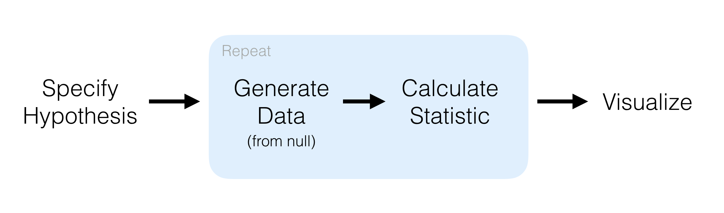
Source: infer package website

Linear models

\[y_i = \beta_0 + \beta_1 x_i + \varepsilon_i\] \[\boldsymbol{\text{y}} = \boldsymbol{\text{X}}^{\text{T}}\boldsymbol{\beta} + \boldsymbol{\varepsilon}\]

The lm() function

lm(formula, data, subset, na.action, ...)

R offers lm() to fit linear models, one of the most fundamental yet powerful tools for statistical modeling. A linear model with a single explanatory variable is called a simple linear model. A linaer model with multiple explanatory variables is called muliple linear regression model.

A model to be fitted is specificed according to the formula input. data is an optional argument, which can take a data frame or one of its variants. If data input is provided, its column names can be used directly in the formula.

R formula

formula <- y ~ x1 + x2

Here we take a closer look at the R formula object.

The response variable is placed on the left-hand side of the tilde symbol (~), and the explanatory variables on the right-hand side.

Adding multiple explanatory variables can be done using + symbol. We can simply use y ~ . to include all other columns additively as expanatory variables.

Model summary

lmfit <- lm(formula, data)

print(lmfit) # not recommended
summary(lmfit)

An output of lm() is an R object of lm class. Simply printing an lm object gives only minimal information on the fitted model.

In order to get a more compresensive model summary, we can we summary() function with a model input (e.g. lm).

Example

We fit a simple linear model with violentCrime as the reponse variable and propertyCrime as the explanatory variable. The class of the fitted model object is lm.

my_lmfit <- lm(violentCrime ~ propertyCrime, ispcrime)
class(my_lmfit)

## [1] "lm"

Here is the output for using the default printing method:

my_lmfit

## 
## Call:
## lm(formula = violentCrime ~ propertyCrime, data = ispcrime)
## 
## Coefficients:
##   (Intercept)  propertyCrime  
##      -79.7683         0.1994

And here is using summary():

summary(my_lmfit)

## 
## Call:
## lm(formula = violentCrime ~ propertyCrime, data = ispcrime)
## 
## Residuals:
##     Min      1Q  Median      3Q     Max 
## -2239.5    -2.2    57.0    78.3  3992.9 
## 
## Coefficients:
##                 Estimate Std. Error t value Pr(>|t|)    
## (Intercept)   -79.768287  16.496961  -4.835 1.77e-06 ***
## propertyCrime   0.199367   0.001059 188.303  < 2e-16 ***
## ---
## Signif. codes:  0 '***' 0.001 '**' 0.01 '*' 0.05 '.' 0.1 ' ' 1
## 
## Residual standard error: 363.5 on 501 degrees of freedom
##   (7 observations deleted due to missingness)
## Multiple R-squared:  0.9861, Adjusted R-squared:  0.986 
## F-statistic: 3.546e+04 on 1 and 501 DF,  p-value: < 2.2e-16

Model diagnostics

plot(lmfit, which = c(1:3, 5), ...)

Base R plot() function has a method for lm objects, which generates the following 6 diagnostics plots:

“Residuals vs Fitted”
“Normal Q-Q”
“Scale-Location”
“Cook’s distance”
“Residuals vs Leverage”
“Cook’s dist vs Leverage \(h_{ii}/(1-h_ii)\)”

The default option only prints the first, second, third and fifth of these plots.

Example

Let’s take a look at all six diagnostic plots for our fitted model:

par(mfrow = c(2,3))
plot(my_lmfit, which = c(1:6))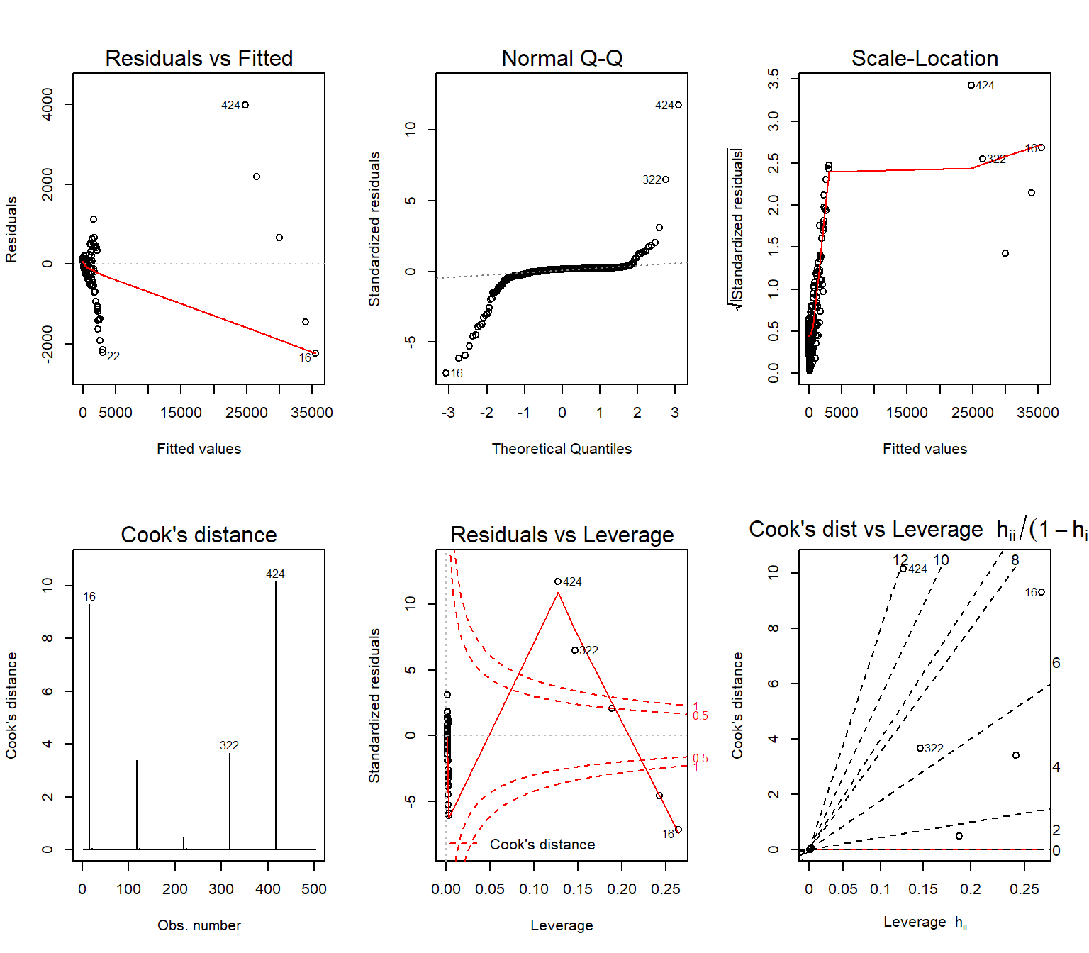

Model evaluation

logLik(object, ...)
AIC(object, ..., k = 2)
BIC(object, ...) # equivalent to AIC with k = log(n)

There are measures of model fit other than \(R^2\). For a model fitted by maximum likelihood algorithm, including the lm model, the following functions are available to get goodness-of-fit measures:

logLik() for log-liklehood value
AIC() for Akaike Information Criterion (with default k)
BIC() for Bayesian Information Criterion

We can read this Wikipedia article for more on maximum likelihood estimation.

Extending lm() formula

A linear model can be extended with simple “tricks” to better fit the data. Four such tricks include:

Transformating model terms
Including interaction terms
Polynomials
Polynomial splines

Transformations

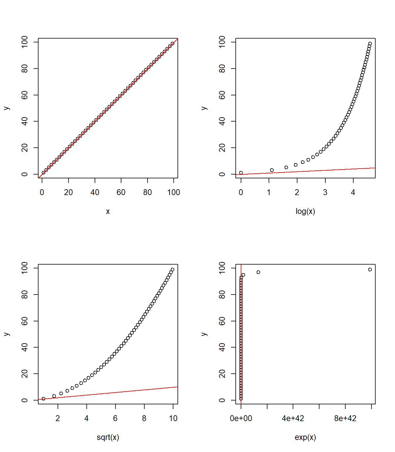
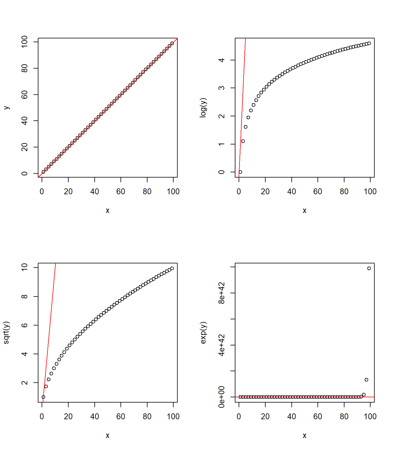
scale(y) ~ log(x1) + sqrt(x2) + ...

We can transform terms on either side of ~ in the formula to get a better model. Common such transformations include:

log(): natural log (cf. log2 and log10)
exp(): exponentiate
sqrt(): square root
scale(): rescale data such that the mean is 0 and the standard deviation is 1

The following two figures offer a visual illustration of the effect of applying some of these transformations.

Transforming `x`

Transforming `y`

Interactions

y ~ x1 + x2 + x1:x2
y ~ x1 * x2

Interaction terms are used to account for any significant interaction between explanatory variables where the effect of one explanatory variable on the response variable depends on the value of another explanatory variable.

In R formula, x1:x2 takes the interactions of all terms in x1 and x2. Additionally, x1*x2 is equivalent to x1:x2 and the original terms x1 and x2.

Please note that it is generally recommended to keep all the original terms if their interaction term is included.

Polynomials

y ~ ploy(x, degree = n)
y ~ x + I(x^2) + I(x^3) + ...

poly() generates the n-th degree polynimals of the input x
ploy(x, 3) is equivalent to using x + I(x^2) + I(x^3)
- I() ensures the ^ with a symbol is used as an arithmetic operator

Polynomial splines

library(splines) # part of R "base pacakges"
y ~ ns(x, ...)
y ~ bs(x, degree = n, ...)

ns() is used for the natural cubic splines
bs() is used for the n-th degree polynomial splines
- equivalent to bs(x, degree = 3)

`broom` package

broom is a tidyverse package for “tidying up” statistical model outputs in R, i.e., converting them into tidy data frames.

Visit broom GitHub repository and “broom as well as dplyr” vignette to learn more about the package.

`broom` functions

glance(x, ...)
tidy(x, ...)
augment(x, ...)

broom is a small package consists of only the following three functions:

glance() takes a model object and returns a concise one-row summary of the model.
tidy() takes a model object and returns a data.frame with the coeffcient estimation results
augment() takes a model object and returns a data.frame for each observation with additional columns such as predictions, residuals and cluster assignments

Example

Let’s try these functions to see how they work. We will use my_lmfit and apply each broom function to the model.

First, we use glance() to see the model summary metrics in a tidy format.

glance(my_lmfit)

##   r.squared adj.r.squared    sigma statistic p.value df    logLik      AIC
## 1 0.9860675     0.9860396 363.4653  35457.96       0  2 -3678.253 7362.506
##        BIC deviance df.residual
## 1 7375.168 66185630         501

Next, tidy returns the model estimates in a tidy format.

tidy(my_lmfit)

##            term    estimate   std.error  statistic      p.value
## 1   (Intercept) -79.7682868 16.49696109  -4.835332 1.771126e-06
## 2 propertyCrime   0.1993675  0.00105876 188.302852 0.000000e+00

And the outputs really are of data.frame class

# check the class of each output
c(class(glance(my_lmfit)), class(glance(my_lmfit)))

## [1] "data.frame" "data.frame"

Finally, we use augment to add to the input data additional columns based on the fitted model:

head(augment(my_lmfit))

##   .rownames violentCrime propertyCrime   .fitted  .se.fit     .resid
## 1         1          218          1555 230.24816 16.26976 -12.248156
## 2         2          119           290 -21.95172 16.44233 140.951715
## 3         3            6           211 -37.70175 16.45666  43.701747
## 4         4           59           733  66.36808 16.36964  -7.368081
## 5         5            7            38 -72.19232 16.48949  79.192322
## 6         6           42           505  20.91229 16.40542  21.087706
##          .hat   .sigma      .cooksd  .std.resid
## 1 0.002003718 363.8282 1.142258e-06 -0.03373209
## 2 0.002046448 363.7739 1.545129e-04  0.38819703
## 3 0.002050017 363.8234 1.487927e-05  0.12035979
## 4 0.002028394 363.8285 4.184743e-07 -0.02029235
## 5 0.002058203 363.8113 4.905554e-05  0.21810593
## 6 0.002037270 363.8274 3.442885e-06  0.05807767

The output is, again, a tidy data.frame object.

class(augment(my_lmfit))

## [1] "data.frame"

`modelr` package

modelr is a tidyverse package that provides helper functions for statistical modeling in R. Its helper functions are designed to facilitate the following:

partitioning and sampling
model quality metrics
interacting with models

You can visit modelr GitHub repository or read the “Model Basics” chapter in R for Data Science to learn more about the package.

Partitioning and sampling

resample(data, idx)
resample_partition(data, p)
bootstrap(data, n, id = ".id")

resample take a data frame and a vector of indices to create a pointer object, which can be either turned into a data frame or used directly in modeling functions (e.g. lm())
resample_partition takes a data and a named numeric vector to specify partitioning. Its output is a list of random partitions.
bootstrap takes a data frame and an integer to specify the number of bootstrap replicates to generate. The output is a data frame of bootstrap samples column and id column

`resample_partition()` example

resample_partition() is suited for creating randomly assigned treatment/control groups. The output is a nested list of partitions. Note that resampling is a “random” process and the output will change each time the code is executed. To ensure reproducibility (i.e. the same result), use set.seed().

set.seed(1) # for reproducibility

partitioned <- ispcrime %>%
  filter(year == "2015") %>%
  resample_partition(p = c(treatment = 0.5, control = 0.5))

partitioned

## $treatment
## <resample [50 x 12]> 1, 2, 5, 10, 11, 12, 14, 16, 19, 22, ...
## 
## $control
## <resample [52 x 12]> 3, 4, 6, 7, 8, 9, 13, 15, 17, 18, ...

Each partition is also a list, which contains data and idx. The former is a data.frame of the partition, the the latter is a numeric vector of indices assigned to the partition.

head(partitioned$treatment$data)

##   year    county violentCrime murder rape robbery aggAssault propertyCrime
## 1 2015     Adams          227      5   39       9        174          1268
## 2 2015 Alexander          107      0    3       3        101           194
## 3 2015      Bond            5      1    0       0          4           130
## 4 2015     Boone            0      0    0       0          0             1
## 5 2015     Brown            9      0    1       0          8            11
## 6 2015    Bureau           53      1   17       4         31           360
##   burglary larcenyTft MVTft arson
## 1      274        944    43     7
## 2       58        119     9     8
## 3       39         84     7     0
## 4        0          0     0     1
## 5        4          5     2     0
## 6      110        244     6     0

partitioned$treatment$idx

##  [1]   1   2   5  10  11  12  14  16  19  22  24  25  26  27  28  30  32
## [18]  34  36  38  39  40  42  44  45  48  50  53  54  55  56  57  58  61
## [35]  64  69  71  75  77  82  84  86  87  91  92  95  97  98  99 100

Model quality metrics

rmse(model, data)
mae(model, data)
qae(model, data, probs = c(0.05, 0.25, 0.5, 0.75, 0.95))
rsquare(model, data)

modelr offers the following functions to quickly extract model quality metrics:

rmse() returns the root mean squared error
mae() returns the mean abosolute error
qae() returns quantiles of absolute error
rsquare() returns the \(R^2\) value, i.e. the variance of the predictions divided by the variance of the reponse

Interacting with models

add_predictions(data, model, var = "pred")
add_residuals(data, model, var = "resid")

add_predictions() adds a new column to a data frame for predicted values based on a model
add_residuals() adds a new column to a data frame for residuals based on a model

Example

Let’s see how add_predictions() and add_residuals() work with an example. To make it easier to view, we first get a subset of ispcrime

ispcrime_subset <- select(ispcrime, year:violentCrime, propertyCrime)

Now we use both functiosn to add prediction and residual columns. Note that the residual values equal true values - predicted values.

ispcrime_subset %>%
  add_predictions(my_lmfit) %>%
  add_residuals(my_lmfit) %>%
  head()

##   year    county violentCrime propertyCrime      pred      resid
## 1 2011     Adams          218          1555 230.24816 -12.248156
## 2 2011 Alexander          119           290 -21.95172 140.951715
## 3 2011      Bond            6           211 -37.70175  43.701747
## 4 2011     Boone           59           733  66.36808  -7.368081
## 5 2011     Brown            7            38 -72.19232  79.192322
## 6 2011    Bureau           42           505  20.91229  21.087706

Generalized linear models

\[\text{E}[\boldsymbol{\text{Y}}] = \mu = g^{-1}(\boldsymbol{\text{X}\beta})\] \[\text{Var}[\boldsymbol{\text{Y}}] = \text{V}[\mu] = \text{V}[g^{-1}(\boldsymbol{\text{X}}\boldsymbol{\beta})]\]

GLM basics

The generalized linear model (GLM) extends the linear model to fit response variables with error distribution other than a gaussian distribution.

Three components of GLM are:

A probability distribution from the exponential family
A linear predictor, \(\eta = \boldsymbol{\text{X}\beta}\)
A link function \(g\), such that \(\text{E}[\boldsymbol{\text{Y}}] = \mu = g^{-1}(\eta)\)

See this Wikipedia article for more on GLM and the model components.

The glm() function

glm(formula, family = gaussian, data, ...)

R offers the glm() function to fit GLM models. glm() uses formula to specify the model. Then, it uses family input to specify the link function \(g\). The default is gaussian(link = "identity"), which corresponds to the linear model.

glm() function returns a glm class object, which has a summary() method to inspect the model estimation results.

`family` objects

The following table lists GLM family options available for glm():

family	Default link function	Use
`gaussian`	`(link = "identity")`	Linear model for continous outcome (ordinary linear regression; OLS)
`binomial`	`(link = "logit")`	Logit model for binary outcome (logistic regression)
`poisson`	`(link = "log"`)	Poisson model for count outcome
`Gamma`	`(link = "inverse")`	…
`inverse.gaussian`	`(link = "1/mu^2")`	…
`quasi`	`(link = "identitiy")`	…
`quasibinomial`	`(link = "logit")`	…
`quasipoisson`	`(link = "log")`	…

Logit model

glm(formula, family = binomial, data, ...)

A logit model, i.e. logistic regression, can be fitted using glm() with family = binomial. The response variable must range between 0 and 1 (an error will be thrown otherwise).

Poisson model

glm(formula, family = poisson, data, ...)

A possion model can be fitted using glm() with family = poisson. Here, the response variable must not include negative values (an error will be thrown otherwise).

Better ways?

There are thrid-party packages to provide additional fuctions and/or different interfaces to existing statistical analysis functions. Although I have little exposure to them, the following two might be worth checking:

psych package. See this package vignette by the package author to learn more about it.
jmv package. See this package documentation page to learn more about it.

Resources

Just as in any previous work module parts, what we have seen in this part is only an introduction tot he topic. The following are some useful resources that would help you to deepen your understanding of the basic statistics in R.

Kabacoff, R. “Statistics”. Quick-R.
Lane D. et al. Online Statistics: A Multimedia Course of Study.
Prabhakaran, S. r-statistics.co.
UCLA Institute for Digital Research and Education. “R”.
University of Cincinnati. “Descriptive analytics”. UC Business Analytic R Programming Guide.
University of Cincinnati. “Predictive analytics”. UC Business Analytic R Programming Guide.
Wollschlaeger, D. RExRepos.
Yau, C. “Elementary Statistics with R”. R Tutorial.

References

Lane D. et al. (n.d.). Online Statistics: A Multimedia Course of Study.
Prabhakaran, S. (n.d.). “Statistic Tests”. r-statistics.co.
tidyverse/broom Github repository
tidyverse/modelr Github repository
University of Cincinnati. UC Business Analytics R Programming Guide
Wikipedia contributors. (2018). “Generalized linear model”. Wikipedia, The Free Encyclopedia.

R Workshop: Module 5 (1)

Bobae Kang

April 18, 2018

Links

Statistical modleing with R (1): Basics of statistical modeling

Basic Descriptive Statistics

Quick summary stats

Example

Numerical variables

Central tendency

Variability

Range

Percentiles

Variance

Shape

Outliers

Categorical variables

Table functions

table() example

prop.table() example

ftable() example

xtabs() example

Basic Inferential Statistics

Student’s t-test

Example

Wilcoxon tests

Analysis of Variance

Example

Other statistical tests

An alternative framework

Linear models

The lm() function

R formula

Model summary

Example

Model diagnostics

Example

Model evaluation

Extending lm() formula

Transformations

Transforming x

Transforming y

Interactions

Polynomials

Polynomial splines

broom package

broom functions

Example

modelr package

Partitioning and sampling

resample_partition() example

Model quality metrics

Interacting with models

Example

Generalized linear models

GLM basics

The glm() function

family objects

Logit model

Poisson model

Better ways?

Resources

References

`table()` example

`prop.table()` example

`ftable()` example

`xtabs()` example

Transforming `x`

Transforming `y`

`broom` package

`broom` functions

`modelr` package

`resample_partition()` example

`family` objects