This page contains the notes for the second part of R Workshop Module 2: R basics, which is part of the R Workshop series prepared by ICJIA Research Analyst Bobae Kang to enable and encourage ICJIA researchers to take advantage of R, a statistical programming language that is one of the most powerful modern research tools.

R Basics (2): Gearing up for data analysis

Now that we have an understanding of the basic building blocks of R programming, we can prepare for conducting data analysis in R. Here we start with learning to work with R data frame, the very essense of tabular data manipulation in R. We will then be introduced to the tidyverse framework and the idea of “tidy” data. Finally, we will discuss some recommended coding styles for R.

R Data Frame

## [1] "Look, a data frame!"

##   column1 column2 column3 column4 column5
## 1      11      12      13      14      15
## 2      21      22      23      24      25
## 3      31      32      33      34      35
## 4      41      42      43      44      45
## 5      51      52      53      54      55

What is a data frame?

A data frame is a tabular representation of data where each column is a vector of some type. You can think of Excel spreadsheets, SPSS tables, etc.!

In R, a data frame exists as a data.frame object, which can be seen as a list of vectors of the same length, but with additional functionalities for data analysis!

Accessing data in a data frame works similarly as in accessing data in a list. In fact, a list can be easily converted into a data frame using as.data.frame() (and vice versa, with as.list()).

Example: ISP crime data

I have created an R package called icjiar, which comes with some sample datasets, including a data frame of ISP UCR data. Let’s take a look.

Inspecting a `data.frame` obejct

First we import icjiar package to make ispcrime dataset available in the global environment.

If you do not have icjiar package installed on your computer yet, remove the hash symbol (#) on the first two lines of the following code chunk and execute it to get the package installed. You will then be able to import the package using library() function. See here for installing and loading packages.

# install.packages("devtools")
# devtools::install_github("bobaekang/icjiar")
library(icjiar)

class(ispcrime)  # the class of ispcrime object is "data.frame"

## [1] "data.frame"

Using the class() function, we find that ispcrime is a data.frame object. Alternatively, using the is.data.frame() function, we can check that ispcrime is indeed a data.frame object.

is.data.frame(ispcrime)  # check if ispcrime is a data.frame; TRUE, as expected

## [1] TRUE

Now, we take a look at the “structure” of ispcrime. str() is a function we use to bring out the sturcutre of an R object. In this case, str() prints that our object is a data frame with 12 variables and shows each variable with its data type as well as first few elements.

str(ispcrime)  # reports the "structure" of the data frame

## 'data.frame':    510 obs. of  12 variables:
##  $ year         : int  2011 2011 2011 2011 2011 2011 2011 2011 2011 2011 ...
##  $ county       : Factor w/ 102 levels "Adams","Alexander",..: 1 2 3 4 5 6 7 8 9 10 ...
##  $ violentCrime : int  218 119 6 59 7 42 13 8 12 1210 ...
##  $ murder       : int  0 0 1 0 0 0 0 0 0 5 ...
##  $ rape         : int  37 14 0 24 1 4 0 1 1 127 ...
##  $ robbery      : int  15 4 0 8 0 3 0 0 0 208 ...
##  $ aggAssault   : int  166 101 5 27 6 35 13 7 11 870 ...
##  $ propertyCrime: int  1555 290 211 733 38 505 56 206 119 5332 ...
##  $ burglary     : int  272 92 58 152 14 90 14 38 41 1384 ...
##  $ larcenyTft   : int  1241 183 147 563 22 405 41 165 71 3756 ...
##  $ MVTft        : int  36 11 5 14 1 8 1 2 3 164 ...
##  $ arson        : int  6 4 1 4 1 2 0 1 4 28 ...

Another way of understanding a data frmae is to print the first few rows. This can be achieved using head(), which prints out the first n rows of the data frame. The default is n = 6.

head(ispcrime, 5)  # returns the first n rows of the data frame (default 6)

##   year    county violentCrime murder rape robbery aggAssault propertyCrime
## 1 2011     Adams          218      0   37      15        166          1555
## 2 2011 Alexander          119      0   14       4        101           290
## 3 2011      Bond            6      1    0       0          5           211
## 4 2011     Boone           59      0   24       8         27           733
## 5 2011     Brown            7      0    1       0          6            38
##   burglary larcenyTft MVTft arson
## 1      272       1241    36     6
## 2       92        183    11     4
## 3       58        147     5     1
## 4      152        563    14     4
## 5       14         22     1     1

There are a few functions to inspect the shape of a data.frame object. First, we can try dim() to get the dimension (number of rows by number of columns) of a data.frame object. nrow() and ncol() return the number of rows and the number of columns of a data.frame object, respectively.

dim(ispcrime)  # returns the dimension of the data frame (row  column)

## [1] 510  12

nrow(ispcrime)  # returns the number of rows in the data frame

## [1] 510

ncol(ispcrime)  # returns the number of columns in the data frame

## [1] 12

Finally, we can use colnames() to obtain a vector of a data.frame object’s column names.

colnames(ispcrime)  # returns a vector containing the column names

##  [1] "year"          "county"        "violentCrime"  "murder"       
##  [5] "rape"          "robbery"       "aggAssault"    "propertyCrime"
##  [9] "burglary"      "larcenyTft"    "MVTft"         "arson"

Accessing desired subsets

Now we explore accessing desired subsets of a data.frame object. We start with columns. The following are three different ways to get the first column of ispcrime, which has the name year:

ispcrime$year # access a column by name
ispcrime[[1]] # access the first column by index
ispcrime[, 1] # yet another way to access the first column!

##   [1] 2011 2011 2011 2011 2011 2011 2011 2011 2011 2011 2011 2011 2011 2011
##  [15] 2011 2011 2011 2011 2011 2011 2011 2011 2011 2011 2011 2011 2011 2011
##  [29] 2011 2011 2011 2011 2011 2011 2011 2011 2011 2011 2011 2011 2011 2011
##  [43] 2011 2011 2011 2011 2011 2011 2011 2011 2011 2011 2011 2011 2011 2011
##  [57] 2011 2011 2011 2011 2011 2011 2011 2011 2011 2011 2011 2011 2011 2011
##  [71] 2011 2011 2011 2011 2011 2011 2011 2011 2011 2011 2011 2011 2011 2011
##  [85] 2011 2011 2011 2011 2011 2011 2011 2011 2011 2011 2011 2011 2011 2011
##  [99] 2011 2011 2011 2011 2012 2012 2012 2012 2012 2012 2012 2012 2012 2012
## [113] 2012 2012 2012 2012 2012 2012 2012 2012 2012 2012 2012 2012 2012 2012
## [127] 2012 2012 2012 2012 2012 2012 2012 2012 2012 2012 2012 2012 2012 2012
## [141] 2012 2012 2012 2012 2012 2012 2012 2012 2012 2012 2012 2012 2012 2012
## [155] 2012 2012 2012 2012 2012 2012 2012 2012 2012 2012 2012 2012 2012 2012
## [169] 2012 2012 2012 2012 2012 2012 2012 2012 2012 2012 2012 2012 2012 2012
## [183] 2012 2012 2012 2012 2012 2012 2012 2012 2012 2012 2012 2012 2012 2012
## [197] 2012 2012 2012 2012 2012 2012 2012 2012 2013 2013 2013 2013 2013 2013
## [211] 2013 2013 2013 2013 2013 2013 2013 2013 2013 2013 2013 2013 2013 2013
## [225] 2013 2013 2013 2013 2013 2013 2013 2013 2013 2013 2013 2013 2013 2013
## [239] 2013 2013 2013 2013 2013 2013 2013 2013 2013 2013 2013 2013 2013 2013
## [253] 2013 2013 2013 2013 2013 2013 2013 2013 2013 2013 2013 2013 2013 2013
## [267] 2013 2013 2013 2013 2013 2013 2013 2013 2013 2013 2013 2013 2013 2013
## [281] 2013 2013 2013 2013 2013 2013 2013 2013 2013 2013 2013 2013 2013 2013
## [295] 2013 2013 2013 2013 2013 2013 2013 2013 2013 2013 2013 2013 2014 2014
## [309] 2014 2014 2014 2014 2014 2014 2014 2014 2014 2014 2014 2014 2014 2014
## [323] 2014 2014 2014 2014 2014 2014 2014 2014 2014 2014 2014 2014 2014 2014
## [337] 2014 2014 2014 2014 2014 2014 2014 2014 2014 2014 2014 2014 2014 2014
## [351] 2014 2014 2014 2014 2014 2014 2014 2014 2014 2014 2014 2014 2014 2014
## [365] 2014 2014 2014 2014 2014 2014 2014 2014 2014 2014 2014 2014 2014 2014
## [379] 2014 2014 2014 2014 2014 2014 2014 2014 2014 2014 2014 2014 2014 2014
## [393] 2014 2014 2014 2014 2014 2014 2014 2014 2014 2014 2014 2014 2014 2014
## [407] 2014 2014 2015 2015 2015 2015 2015 2015 2015 2015 2015 2015 2015 2015
## [421] 2015 2015 2015 2015 2015 2015 2015 2015 2015 2015 2015 2015 2015 2015
## [435] 2015 2015 2015 2015 2015 2015 2015 2015 2015 2015 2015 2015 2015 2015
## [449] 2015 2015 2015 2015 2015 2015 2015 2015 2015 2015 2015 2015 2015 2015
## [463] 2015 2015 2015 2015 2015 2015 2015 2015 2015 2015 2015 2015 2015 2015
## [477] 2015 2015 2015 2015 2015 2015 2015 2015 2015 2015 2015 2015 2015 2015
## [491] 2015 2015 2015 2015 2015 2015 2015 2015 2015 2015 2015 2015 2015 2015
## [505] 2015 2015 2015 2015 2015 2015

Accessing select rows of a data.frame is somewhat simpler:

ispcrime[1, ]  # access the first row by index

##   year county violentCrime murder rape robbery aggAssault propertyCrime
## 1 2011  Adams          218      0   37      15        166          1555
##   burglary larcenyTft MVTft arson
## 1      272       1241    36     6

Combining these two, we can get to a particular cell in a data.frame object.

# access a specific cell (first row of the first column)
ispcrime$year[1]
ispcrime[[1]][1]
ispcrime[1, 1]

## [1] 2011

Creating a data.frame object

Most often, we will be working with data.frame objects that result from importing external datasets or come as part of imported packages. Sometimes, however, we need to create a data.frame object. There are two main ways to do so:

Using data.frame(): Here, we either use vector objects as argument inputs or simultanesouly create vectors and assign column names to them.
Coercing a list using as.data.frame(): We can also convert an existing list object into a data.frame object.

Using data.frame()

Using existing vectors

fruits <- c("apple", "banana", "clementine")
animals <- c("dogs", "cats", "llamas")
icecream_flavors <- c("chocolate", "vanila", "cookie dough")

df1 <- data.frame(fruits, animals, icecream_flavors)

print(df1)

##       fruits animals icecream_flavors
## 1      apple    dogs        chocolate
## 2     banana    cats           vanila
## 3 clementine  llamas     cookie dough

Simultaneously creating vectors and assigning names

df2 <- data.frame(
  fruits = c("apple", "banana", "clementine"),
  animals = c("dogs", "cats", "llamas"),
  icecream_flavors = c("chocolate", "vanila", "cookie dough")
)

print(df2)

##       fruits animals icecream_flavors
## 1      apple    dogs        chocolate
## 2     banana    cats           vanila
## 3 clementine  llamas     cookie dough

Converting a list using as.data.frame()

lt <- list(
  fruits = c("apple", "banana", "clementine"),
  animals = c("dogs", "cats", "llamas"),
  icecream_flavors = c("chocolate", "vanila", "cookie dough")
)

df3 <- as.data.frame(lt)

print(df3)

##       fruits animals icecream_flavors
## 1      apple    dogs        chocolate
## 2     banana    cats           vanila
## 3 clementine  llamas     cookie dough

Transforming a `data.frame` object

It is common to find that the given data.frame object is not exactly in the desired shape or form. Here we will take a quick look at the following four basic operations for transforming a data.frame object:

change column names
add / modify / remove columns
add / modify / remove rows
modify cell values

Change column names

colnames(df1) <- c("my_fruits", "my_animals", "my_flavors")

print(df1)

##    my_fruits my_animals   my_flavors
## 1      apple       dogs    chocolate
## 2     banana       cats       vanila
## 3 clementine     llamas cookie dough

Add columns

Adding new columns can be done in two ways. First, we can use one of the methods to access a column but with a slight twist: this time, we point to a non-existing column and assign a vector to it. Second, we can use the cbind() function, which takes an existing data.frame object and a vector as its arguments and returns a new data.frame object now with an additional column.

# using $ index
df1$my_colors <- c("red", "green", "orange")

# using cbind() function
my_cities <- c("Chicago", "New Work", "Los Angeles")
df1 <- cbind(df1, my_cities)

print(df1)

##    my_fruits my_animals   my_flavors my_colors   my_cities
## 1      apple       dogs    chocolate       red     Chicago
## 2     banana       cats       vanila     green    New Work
## 3 clementine     llamas cookie dough    orange Los Angeles

It must be noted that, in the example above, the length of both vectors for my_colors and my_cities had to match the number of columns in the existing data.frame obejct, df1. Otherwise, R will throw an error.

Also, when adding columns in the first way, we must be careful not to leave “holes” after existing columns. For example, if we try df1[, 10] <- c(1,2,3), R will throw an error because the df1 cannot have the tenth column without already having the ninth column.

Modify columns

Modifying existing columns is very similar to adding ones, except that we assign a new vector to overwrite an existing column. Also, note that we can use NA to give a missing value to certian cells.

df1[["my_colors"]] <- c("maroon", "blue", "purple")
df1$my_cities <- c("Chicago", NA, "Paris")

df1

##    my_fruits my_animals   my_flavors my_colors my_cities
## 1      apple       dogs    chocolate    maroon   Chicago
## 2     banana       cats       vanila      blue      <NA>
## 3 clementine     llamas cookie dough    purple     Paris

Remove columns

There are two major ways to remove columns. First, we can point to a specific column and assign NULL to it. Alternatively, we can take a subset of the columns and reassign it to the object.

# assinging NULL
df1$my_colors <- NULL

df1

##    my_fruits my_animals   my_flavors my_cities
## 1      apple       dogs    chocolate   Chicago
## 2     banana       cats       vanila      <NA>
## 3 clementine     llamas cookie dough     Paris

# subsetting
df1 <- df1[, 1:3]  # or c("my_fruits", "my_animals", "my_flavors")

df1

##    my_fruits my_animals   my_flavors
## 1      apple       dogs    chocolate
## 2     banana       cats       vanila
## 3 clementine     llamas cookie dough

Add rows

Compared to columns, working with rows of a data.frame object is more limited.

Adding rows can be done by the rbind() function, which works similarly to how the aforementioned cbind() does.

new_row <- data.frame(
  my_fruits = "strawberry",
  my_animals = "monkeys",
  my_flavors = "butter pecan"
)
df1 <- rbind(df1, new_row)

df1

##    my_fruits my_animals   my_flavors
## 1      apple       dogs    chocolate
## 2     banana       cats       vanila
## 3 clementine     llamas cookie dough
## 4 strawberry    monkeys butter pecan

Remove rows

An easy way to remove rows from a data.frame object is taking a subset and reassigning that to the object.

# subsetting
df1 <- df1[1:3, ]

df1

##    my_fruits my_animals   my_flavors
## 1      apple       dogs    chocolate
## 2     banana       cats       vanila
## 3 clementine     llamas cookie dough

Modify cells

Modifying individual sells is not much different. However, we must make sure that the new element we would like to give to a cell is of the same type as the existing column. It is noteworthy that, when we create a data.frame, a character vector becomes a factor type by default (this default behavior can be changed with the stringsAsFactors argument of data,frame()). Therefore, the following will fail.

# this doesn't work ... why?
df1$my_flavors[1] <- "mint chocolate chip"

## Warning in `[<-.factor`(`*tmp*`, 1, value = structure(c(NA, 3L, 2L), .Label
## = c("chocolate", : invalid factor level, NA generated

df1

##    my_fruits my_animals   my_flavors
## 1      apple       dogs         <NA>
## 2     banana       cats       vanila
## 3 clementine     llamas cookie dough

# because the column is a factor and only
# new values of the existing levels can be added
df1$my_flavors

## [1] <NA>         vanila       cookie dough
## Levels: chocolate cookie dough vanila butter pecan

In such a case, we can first coerce the target column into a desired data type and then modify the cell.

# first we coerce the column into character class
df1$my_flavors <- as.character(df1$my_flavors)

# now works!
df1$my_flavors[1] <- "mint chocolate chip"

df1

##    my_fruits my_animals          my_flavors
## 1      apple       dogs mint chocolate chip
## 2     banana       cats              vanila
## 3 clementine     llamas        cookie dough

You may encounter a similar issue when trying to give a numeric type value to an integer column. Make sure the data types match!

Extending data frame

In practice, R’s original data.frame is rarely used since better alternatives are available. There are two prominant alternatives:

tibble
data.table

It is noteworthy that both alternatives are in fact extensions of the original data.frame. Consequently, either can be manipulated using methods for a data.frame objects.

`tibble`

## # A tibble: 5 x 5
##   column1 column2 column3 column4 column5
##     <dbl>   <dbl>   <dbl>   <dbl>   <dbl>
## 1     11.     12.     13.     14.     15.
## 2     21.     22.     23.     24.     25.
## 3     31.     32.     33.     34.     35.
## 4     41.     42.     43.     44.     45.
## 5     51.     52.     53.     54.     55.

tibble is a part of the tidyverse framework (we’ll come back to this). A tibble object follows easily understood tidyverse syntax and has a refined print method, which can be seen as more informative and convenient. Coercing a data.frame object into a tibble can be done with as_tibble() from the tibble package.

Please see here for more on tibble.

`data.table`

##    column1 column2 column3 column4 column5
## 1:      11      12      13      14      15
## 2:      21      22      23      24      25
## 3:      31      32      33      34      35
## 4:      41      42      43      44      45
## 5:      51      52      53      54      55

data.frame objects are made available via the data.table package. It is highly optimized for larger tables (e.g. >100K rows) and provides compact syntax for advanced slicing and dicing of tablular data. Coercing a data.frame object into a data.table can be done with as.data.table().

See here for more on data.table.

R Add-On Packages

Source: DataCamp

What are add-on packages?

The capabilities of R are extended through user-created packages, which allow specialized statistical techniques, graphical devices, import/export capabilities, reporting tools […], etc. - “R (programming language)”, Wikipedia

Using packages

To use an add-on package, we first have to install it using, for example, the install.packages() function. Onces the package is installed, it can be imported to the global environment using library().

# first we should install the desired package
install.packages("some_package")

# then we import the package to use its functionalities
library(some_package)

Two ways of installing packages

There are in fact two ways to install new packages.

From CRAN (Comprehensive R Archive Network):
- Packages that are listed on CRAN are tested and can be trusted. In other words, they are generally more robust towards bugs. We can install a pacakge from CRAN using install.packages("package").
From specific Github repositories (i.e., development versions):
- If we want the latest version of a package with cutting-edge features, we may choose to install the package using the install_github("author/package") method, which will pull the most up-to-date version of the package as shown in its GitHub repository. The install_github() function is available via the devtools package.

Also, check out “Install Packages” tutorial video by RStudio, Inc.

Tidyverse Framework

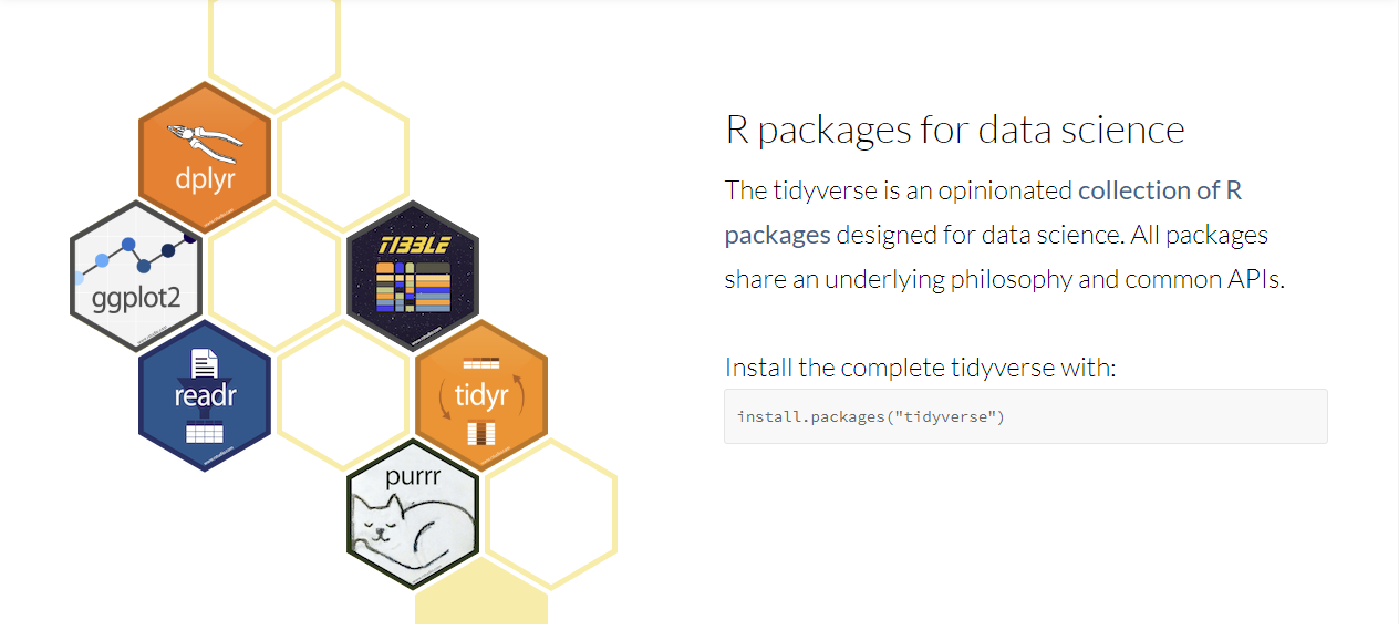
Source: tidyverse.org

tidyverse is a set of packages that are based on a particular perspective on working with data in R. It is also one of the most popular styles of doing data analysis.

Tidy approach to data science

“The tidyverse framework” introduces the notion of tidy data. A dataset is tidy if:

Each variable is in a column

Each observation is a row

Each value is a cell.

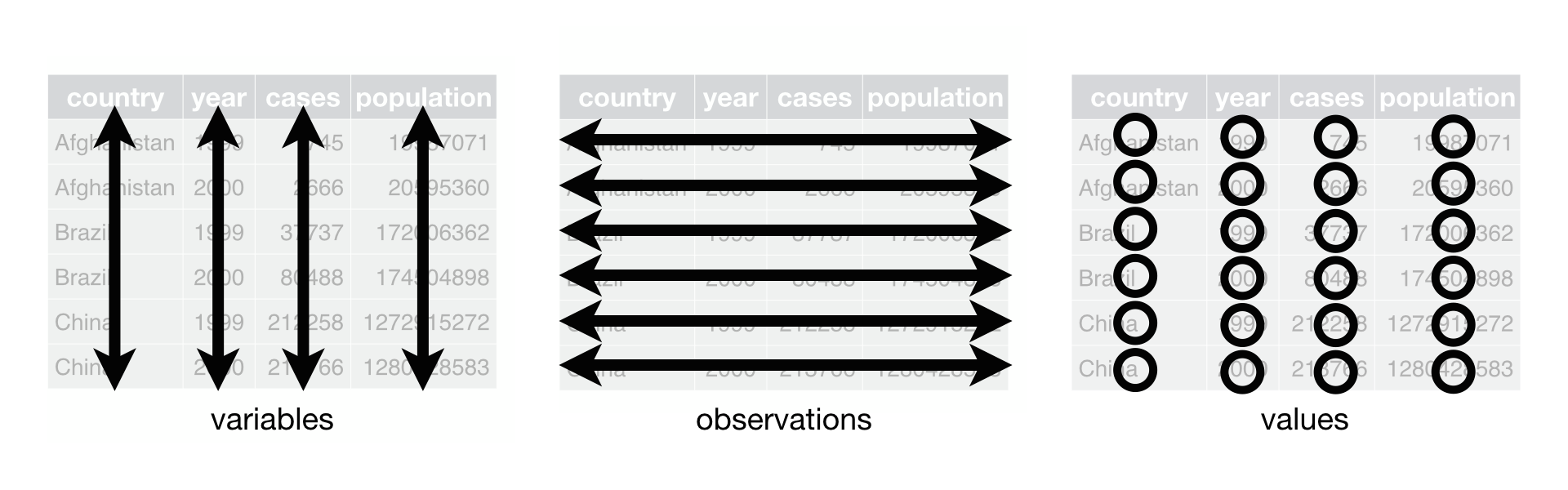
Source: Hadley Wickham, 2017, R for Data Science

See here for more on tidy data

Untidy data?

Anything that does not follow the aforementioned principles of a tidy dataset can be thought untidy:

Multiple variables in a single column
Multiple observations in a single row
Multiple rows for a single observation
Multiple values in a single cell
Multiple cells for a single value

Untidy example 1

## 
## Attaching package: 'dplyr'

## The following objects are masked from 'package:stats':
## 
##     filter, lag

## The following objects are masked from 'package:base':
## 
##     intersect, setdiff, setequal, union

##      year/county violentCrime/propertyCrime
## 1     2011/Adams                   218/1555
## 2 2011/Alexander                    119/290
## 3      2011/Bond                      6/211
## 4     2011/Boone                     59/733
## 5     2011/Brown                       7/38
## 6    2011/Bureau                     42/505

Untidy example 2

##    index year    county typeViolent valueViolent
## 1      1 2011     Adams      murder            0
## 2      1 2011     Adams        rape           37
## 3      1 2011     Adams     robbery           15
## 4      1 2011     Adams  aggAssault          166
## 5      2 2011 Alexander      murder            0
## 6      2 2011 Alexander        rape           14
## 7      2 2011 Alexander     robbery            4
## 8      2 2011 Alexander  aggAssault          101
## 9      3 2011      Bond      murder            1
## 10     3 2011      Bond        rape            0

Tidyverse core packages

ggplot2 for data visualization
dplyr for data manipulation
tidyr for creating “tidy data”
readr for data import/export
purrr for loop operations
tibble for data representation

Resources

RStudio, Inc., “tidy tutorial” video

Good Code, Bad Code

Source: The New York Times

Why style guide?

The goal [of the style guide] is to make our R code easier to read, share, and verify.
- Google’s R Style guide

The key benefits of following a style guide include:

Readability
Productivity
Reproducibility

Which style guide?

Currently, there is no single style guide adopted by the R community as the standard. However, there are two style guides that are considered authoritative:

Personal recommendations

I recommand anyone who are picking up R to start with the tidyverse style guide, which is suggested by one of the most influential personalities in R community, Hadley Wickham, and most widely adopted.

You may consider adding extra rules only if they will help your team to better collaborate and maintain code. Even then, you should keep the changes to minimum so that code remains accessible to others, including future teammates and even your future self!

In the following, I will offer some key elements of the tidyvese style guide:

Object naming

Be descriptive yet concise
- somewhat dependent on the shared knowledge on the subject matter
Use underscore for names consisting of multiple words
Nouns for variables, verbs for functions
Avoid re-using common names for functions and variables
- Using “reserved words” to assign objects will throw errors

Naming a variable (e.g. for firearm arrests)

# Good
firearm_arr
fa_arr

# Bad
arrests_with_firearm_charges  # too verbose
firearmArrests                # violating underscore convention
FireArm_Arrests               # mixing underscore with other way of naming
farr                          # not descriptive enough
x                             # not descriptive at all

Naming a function (e.g. for counting arrests)

# Good
count_arr <- function(x) { ... }

# Bad
num_arr <- function(x) { ... }  # noun for a function
do_arr  <- function(x) { ... }  # not descriptive enough
count   <- function(x) { ... }  # too generic (common name)

Reserved words in R

if else repeat while function for  
in next break  # used in loops, conditions, functions

TRUE FALSE  # logical values

NULL  # undefined

Inf  # infinity

NaN  # Not a Number

NA  # not available (missing)

NA_integer_ NA_real_
NA_complex_ NA_character_  # NA for atomic vector types

...  # dot method for one function to pass arguments to another

Whitespaces for readable code

Add a space
- around operators (+, -, <, =, etc.)
  - Exceptions include :, ::, and :::
- after a comma (but not before–like in regular English)
- before a left paranthesis (, except when it is a function call
Extra spacing for alignment of code
Indentation for clarifying hierarchy

Adding spaces

# Good
greetings <- paste("Hello", "World!", sep = " ")
df[2, ]
x <- 1:10 
base::Random() # calling a function with specifying the package

# Bad
greetings<-paste("Hello","world!",sep="")
df[ 2,]
x<- 1 : 10
base :: Random ()

Extra spacing

# for aligning function arguments
some_function (
  first_argument   = value_1
  another_argument = value_2
  example          = value_3
)

# for aligning variable assignments
numbers        <- c(1, 2, 3)
roman_numerals <- c("I", "II", "III")
letters        <- c("a", "b", "c")

Indentation

# Good
if (x > 0) {
  i = 0
  while (i < 10) {
    message("Wait, I'm in a loop")  
    i <- i + 1
  }
  message("x is positive.")
} else {
  message("x is not positive")
}

# Bad
if (y > 0) {
    j = 0
while (j < 10) {
message("Wait, I'm in a loop")  
j <- j + 1
    }
      message("y is positive.")
} else {
message("y is not positive")
}

Comments for intelligible code

Use comments (words after the # symbol) for clarification
- add two spaces before starting a comment if the comment comes after an expression
However, whenever possible, use descriptive names to reduce the need for clarification and avoid verbosity!
Example of unnecesary comment:

# the following code calculates the average of some numbers
numbers <- c(1, 3, 5)  # assign a vector of numbers to numbers object
average <- sum(numbers) / length(numbers)  # divide the sum of numbers vecotr by its length to get the average

Most importantly…

Be consistent!
Be concise!
Be clear!

Finally, remember that the ultimate goal of adopting a particular coding style to facilitate your work.

References

Google. (n.d.). “Google’s R Style Guide”.
Grolemund, G. & Wickham, H. (2017). R for Data Science.
Wickham, H. (n.d.). “The tidyverse style guide”.

R Workshop: Module 2 (2)

Bobae Kang

March 22, 2018

Links