This page contains the notes for the first part of R Workshop Module 3: Data Analysis with R, which is part of the R Workshop series prepared by ICJIA Research Analyst Bobae Kang to enable and encourage ICJIA researchers to take advantage of R, a statistical programming language that is one of the most powerful modern research tools.

Data Analysis with R (1): Getting started with `tidyverse`

Source: tidyverse.org

In Module 3, we will be exploring several tidyverse packages that offer powerful functionalities for data analysis.

Getting Ready

Installing the packages

tidyverse is a set of R packages as well as an opinionated philosophy underlying these packages on how the practice of working with data in R should be. Although it is not the only way of working with data in R, tidyverse packages have become highly popular among R users.

Installing all tidyverse packages can be easily done with the follwoing command:

# Install from CRAN
install.packages("tidyverse")

# Or the development version from GitHub
# install.packages("devtools")
devtools::install_github("hadley/tidyverse")

Installing tidyverse package installs the following:

core tidyverse packages
- ggplot2, dplyr, tidyr, readr, purrr, tibble
packages to work with specific vector types
- hms, stringr, lubridate, forcats
packages to import data
- feather, haven, httr, jsonlite, readxl, rvest, xml2
packages to facilitate statistical modeling
- modelr, broom

Alternatively, each pacakge can be installed separately:

# Install ggplot2
install.packages("ggplot2")

# Install both dplyr and tidyr with a single commend
#   with a character vector of the package names 
install.packages(c("dplyr", "tidyr"))

Importing the packages

Once installed, we can now import the packages using library():

# This imports the core tidyverse packages
library(tidyverse)

# Or import packages separately
library(dplyr)
library(tidyr)

In the following, we will explore two powerful tidyverse packages for wrangling tabluar data, dplyr and tidyr.

Manipulating Your Data

Source: tidyverse.org

Key dplyr functions

In this section, we will learn the following dplyr functions:

arange()
select() rename()
filter()
mutate() transmute()
left_join()
summarise()
group_by() ungroup()
%>%, the pipe operator

Please note that this section is not intended to be an exhaustive documentation and description of the listed functions–or dplyr package for that matter. For more information, please check out the reference materials listed below.

Sort rows by variables

arrange(tbl, ...)

arrange() is used to sort the rows by a selection of column variables. The first argument of arrange() is a tabular data object. In fact, as we will see soon, almost all other functions of tidyverse packages take a data object as the first input. This tabular data can be of the data.frame class or any of its extensions, such as tidyverse’s very own tibble class.

arrange() takes columns by which to sort the data as additional arguments. If multiple columns are provided, the sorting taks place in a hierarchical manner: the data is first sorted by the first column, then by the second column, and so on. By default, sorting is in an ascending order (smaller to larger). Sorting in a descending order can be done by wrapping the column with desc().

Example

The following example sorts, or arranges, the ispcrime data by the county column. To make it manageable, we also use the head() to print only the first few rows:

# without using pipe
head(arrange(ispcrime, county))

# with using pipe
ispcrime %>%
  arrange(county) %>%
  head()

##   year    county violentCrime murder rape robbery aggAssault propertyCrime
## 1 2011     Adams          218      0   37      15        166          1555
## 2 2012     Adams          205      0   28      16        161          1587
## 3 2013     Adams          222      1   33      21        167          1564
## 4 2014     Adams          222      2   34      13        173          1550
## 5 2015     Adams          227      5   39       9        174          1268
## 6 2011 Alexander          119      0   14       4        101           290
##   burglary larcenyTft MVTft arson
## 1      272       1241    36     6
## 2      287       1261    30     9
## 3      297       1204    55     8
## 4      305       1201    39     5
## 5      274        944    43     7
## 6       92        183    11     4

As shown above, there are two ways to work with dplyr functions:

Traditional syntax for using R functions
Using pipe operators, %>%

We will take a closer look at %>% below. In the meantime, it is sufficient to note that the object before %>% is fed, or “piped,” into the following function as the input for its first argument.

The folloiwng code illustrates using desc() to sort in a descending order:

# sort by county, in a DESCENDING order
ispcrime %>%
  arrange(desc(county), desc(year)) %>%
  head()

##   year    county violentCrime murder rape robbery aggAssault propertyCrime
## 1 2015  Woodford           29      0    5       0         24           227
## 2 2014  Woodford           25      0    4       0         21           283
## 3 2013  Woodford           17      0   10       2          5           349
## 4 2012  Woodford           23      0    3       1         19           405
## 5 2011  Woodford           15      1    4       0         10           350
## 6 2015 Winnebago         2692     22  197     563       1910          8279
##   burglary larcenyTft MVTft arson
## 1       35        186     6     0
## 2       50        218    13     2
## 3       81        257    11     0
## 4       65        329    10     1
## 5       90        247    10     3
## 6     1958       5635   618    68

Filter rows with conditions

filter(tbl, ...)

filter() is used to filter data to keep rows that match given conditions. As in arrange(), the first argument is a tabular data object. Conditional expressions to filter data, which should evaluate as TRUE or FALSE for each row, are given as additional arguments.

Example

The following code filters ispcrime to return a subset of data where year value matches 2015 AND murder value is greater than 0. As before, we use head() to show only the first few rows.

ispcrime %>%
  filter(
    year == 2015,
    murder > 0
  ) %>%
  head()

##   year    county violentCrime murder rape robbery aggAssault propertyCrime
## 1 2015     Adams          227      5   39       9        174          1268
## 2 2015      Bond            5      1    0       0          4           130
## 3 2015    Bureau           53      1   17       4         31           360
## 4 2015 Champaign          918      7  127     205        579          5568
## 5 2015     Coles          173      1   33      14        125           632
## 6 2015      Cook        28791    534 1911   11217      15129        124784
##   burglary larcenyTft MVTft arson
## 1      274        944    43     7
## 2       39         84     7     0
## 3      110        244     6     0
## 4     1100       4235   196    37
## 5      146        463    13    10
## 6    20550      90675 12547  1012

Select and/or rename variables

select(tbl, ...)
rename(tbl, ...)

select() and rename() both take a tabular data object as the first argument input. The following arguments are columns to select or rename. These two functions are quite similar to each other, except that select() returns the selected columns only while rename() keeps all columns.

It is actually possible to renaming each selected column with select() as well. select() can be also used to exclude a section of columns using a minus (-) sign while keeping the rest.

Example

Let’s take a look at an example on how to use select() to select columns, with changing their names in certain cases. The following code select four columns of ispcrime while changing the names of violentCrime and propertyCrime columns.

# select with renaming columns
ispcrime %>%
  select(year, county, v_crime = violentCrime, p_crime = propertyCrime) %>%
  head()

##   year    county v_crime p_crime
## 1 2011     Adams     218    1555
## 2 2011 Alexander     119     290
## 3 2011      Bond       6     211
## 4 2011     Boone      59     733
## 5 2011     Brown       7      38
## 6 2011    Bureau      42     505

As noted earlier, select() can be used to exclude certain columns. The following code selects all columns of ispcrime except violentCrime and propertyCrime:

# excluding columns
ispcrime %>%
  select(-violentCrime, -propertyCrime) %>%
  head()

##   year    county murder rape robbery aggAssault burglary larcenyTft MVTft
## 1 2011     Adams      0   37      15        166      272       1241    36
## 2 2011 Alexander      0   14       4        101       92        183    11
## 3 2011      Bond      1    0       0          5       58        147     5
## 4 2011     Boone      0   24       8         27      152        563    14
## 5 2011     Brown      0    1       0          6       14         22     1
## 6 2011    Bureau      0    4       3         35       90        405     8
##   arson
## 1     6
## 2     4
## 3     1
## 4     4
## 5     1
## 6     2

Transform and add variables

transmute(tbl, ...)
mutate(tbl, ...)

transmute() and mutate() both take a tabular data object as the first argument input. The following arguments are expressions to transform existing columns or add new ones. An exisiting column is modified with an expression with the same column name. On the other hand, a new column is created with an expression having a new column name.

As with select() and rename(), the two functions here are quite similar to each other, except that transmute() returns the trasnformed/aded columns only while mutate() keeps all columns.

Example

The following code adds a new column named totalCrime, whose value equals the sum of violentCrime and propertyCrime values:

ispcrime %>%
  mutate(totalCrime = violentCrime + propertyCrime) %>%
  head()

##   year    county violentCrime murder rape robbery aggAssault propertyCrime
## 1 2011     Adams          218      0   37      15        166          1555
## 2 2011 Alexander          119      0   14       4        101           290
## 3 2011      Bond            6      1    0       0          5           211
## 4 2011     Boone           59      0   24       8         27           733
## 5 2011     Brown            7      0    1       0          6            38
## 6 2011    Bureau           42      0    4       3         35           505
##   burglary larcenyTft MVTft arson totalCrime
## 1      272       1241    36     6       1773
## 2       92        183    11     4        409
## 3       58        147     5     1        217
## 4      152        563    14     4        792
## 5       14         22     1     1         45
## 6       90        405     8     2        547

If it were with transmute(), the result would include only the totalCrime column.

Merge tables

left_join(tbl1, tbl2, by = NULL, ...)

left_join() takes two tabular data objects to join as the first two arguments. by takes a chracter vector containing a selection of variables to join tables by. By default, all columns with common names are used. The ouput is a merged table where the columns in the second table is added to the first table as new columns where the values of by columns match.

left_join() is named so because it keeps all observations in the first (left) table. There, in fact, are other types of joins including: inner_join(), right_join(), full_join(), semi_join(), and anti_join().

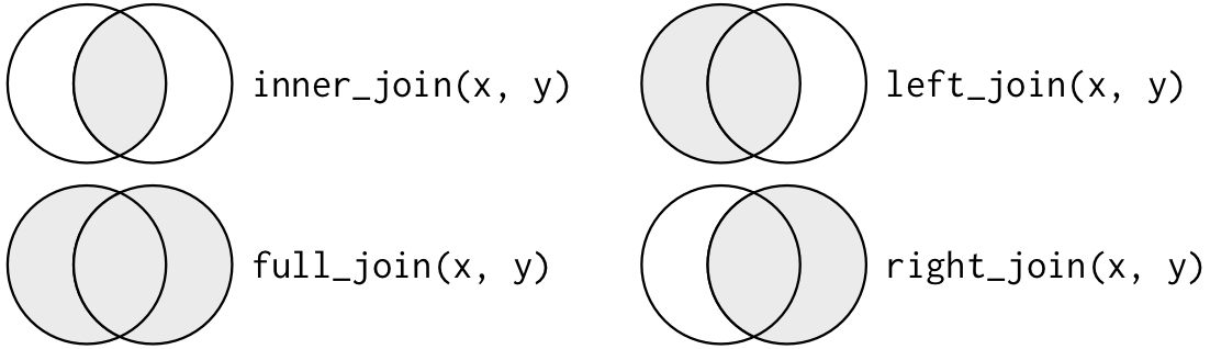
The following four Venn diagrams show how different types of join compare to one another in terms of the observations (rows):

Source: Wickham, H. (2017). R for Data Science

Example

The following code left-joins regions table to ispcrime table on the county values. The regions table has two columns: region and county. Accordingly, the final output is basically the ispcrime table with one extra column, region, that corresponds to the county value:

ispcrime %>%
  left_join(regions, by = "county") %>%
  head()

##   year    county violentCrime murder rape robbery aggAssault propertyCrime
## 1 2011     Adams          218      0   37      15        166          1555
## 2 2011 Alexander          119      0   14       4        101           290
## 3 2011      Bond            6      1    0       0          5           211
## 4 2011     Boone           59      0   24       8         27           733
## 5 2011     Brown            7      0    1       0          6            38
## 6 2011    Bureau           42      0    4       3         35           505
##   burglary larcenyTft MVTft arson   region
## 1      272       1241    36     6  Central
## 2       92        183    11     4 Southern
## 3       58        147     5     1 Southern
## 4      152        563    14     4 Northern
## 5       14         22     1     1  Central
## 6       90        405     8     2  Central

Aggregate and summarise rows

summarise(tbl, ...)
summarize(tbl, ...)

summarise() and summairze() are identical except who they are spelled. This is because the original package author, Hadly Wickham, is an Australian and wrote the names accordingly. Later, due to the demand from American programmers, summarize() was added.

summarise() takes a tabular data object as its first argument, and the following arguments are expressions to “summarize” data. Each of these expressions creates a summary column, which can be given a name just as in the case of transmute() or mutate().

Example

Here, we use summarise() to get the average count of violentCrime and propertyCrime, which are named violentCrimeAverage and propertyCrimeAverage respectively:

ispcrime %>%
  summarise(
    violentCrimeAverage = mean(violentCrime, na.rm = TRUE),
    propertyCrimeAverage = mean(propertyCrime, na.rm = TRUE)
  )

##   violentCrimeAverage propertyCrimeAverage
## 1            500.9702             2912.905

Group by variables

group_by(tbl, ...)
ungroup(tbl, ...)

group_by is a powerful function that allows us to manipulate a data object in “groups,” which is defined by the discrete values in a column, or a selection of columns. As in other dplyr functions, the first argument is a tabular object. The following arguments are columns by which to group the data.

group_by() and ungroup() are the opposite operations. group_by() creates a data object with groups. ungroup() removes the groups.

Example

The following example shows how a groupd data table looks like:

ispcrime %>%
  group_by(year)

## # A tibble: 510 x 12
## # Groups:   year [5]
##     year county violentCrime murder  rape robbery aggAssault propertyCrime
##    <int> <fct>         <int>  <int> <int>   <int>      <int>         <int>
##  1  2011 Adams           218      0    37      15        166          1555
##  2  2011 Alexa~          119      0    14       4        101           290
##  3  2011 Bond              6      1     0       0          5           211
##  4  2011 Boone            59      0    24       8         27           733
##  5  2011 Brown             7      0     1       0          6            38
##  6  2011 Bureau           42      0     4       3         35           505
##  7  2011 Calho~           13      0     0       0         13            56
##  8  2011 Carro~            8      0     1       0          7           206
##  9  2011 Cass             12      0     1       0         11           119
## 10  2011 Champ~         1210      5   127     208        870          5332
## # ... with 500 more rows, and 4 more variables: burglary <int>,
## #   larcenyTft <int>, MVTft <int>, arson <int>

Now, let’s see how group_by() can be used in combination with another dplyr function. In the following, we group our data by year values and get summaries (average crime counts) for each year:

ispcrime %>%
  group_by(year) %>%
  summarise(
    violentCrimeAverage = mean(violentCrime, na.rm = TRUE),
    propertyCrimeAverage = mean(propertyCrime, na.rm = TRUE)
  )

## # A tibble: 5 x 3
##    year violentCrimeAverage propertyCrimeAverage
##   <int>               <dbl>                <dbl>
## 1  2011                538.                3329.
## 2  2012                520.                3192.
## 3  2013                503.                2940.
## 4  2014                464.                2609.
## 5  2015                478.                2481.

Chain operations

We have been using the pipe operator, %>%, in our code examples. Now is a good time to take a closer look at it.

data %>% function1(arg2, ...) %>% ...

%>% is a binary operator that requires two objects for it to work on. Think of + as another example of a binary operator. In the case of %>% the object preciding the operator has to be the first argument for the function that follows the oprator. In other words, the preceding object is injected into the following function as its first argument. The result of the %>% operator is the output of the function.

In fact, as we have already seen before, multiple functions can be chained, or “piped,” using %>% as long as the output of the first “piping” generates a suitable object for the first argument of the next function to be chained.

with piping, we can have a coding style that is cleaner and more intuitive–that reflects the way we think about how we apply the operations to the object, rather than the tranditional syntax where the function that acts on the last comes at the beginning of the statement:

# piping style
object %>%
  function1(arguments1) %>%
  function2(arguments2) %>%
  function3(arguments3)


# traditional style
function3(
  function2(
    function1(
      object,
      arguments1
    ),
    arguments2
  ),
  arguments3  
  
)

# or
function3(function2(function1(object, arguments1), arguments2), arguments3)

`dplyr` in action

Let’s take a look at more concrete examples of using dplyr functions to work on data manipulation and analysis. For those of you who were there at my presentation for the February R&A meeting, these are the some of the examples used in that presentation–now we can understand them better!

Example 1

ispcrime %>%
  filter(substr(county, 1, 1) == "D", year %in% c(2014, 2015)) %>%
  mutate(totalCrime = violentCrime + propertyCrime) %>%
  select(year, county, totalCrime)

##   year  county totalCrime
## 1 2014 De Kalb       2218
## 2 2014 De Witt        182
## 3 2014 Douglas        116
## 4 2014 Du Page      12576
## 5 2015 De Kalb       2173
## 6 2015 De Witt        140
## 7 2015 Douglas        173
## 8 2015 Du Page      12538

In this example, we we want to answer the following question: What are the total crime count in 2014 and 2015 for counties whose name starts with letter D?

We start with ispcrime data
We use the pipe operator to feed the ispcrime data into filter()
- we have two filtering conditions. First condition is that the first letter of the county column value matches “D” (substr(county, 1, 1) == "D")
- Second condition is that the year column value has to be either 2014 or 2015 (year %in% c(2014, 2015))
We use the pipe operator to feed the filtered data into mutate()
- Here we create a new column named totalCrime, which is the sume of violentCrime and propertyCrime values
Finally, we use the filtered and mutated data into select()
- The final output will include year, county, and totalCrime columns only.

Example 2

ispcrime %>%
  left_join(regions) %>%
  group_by(region, county) %>%
  summarise(annualAvgCrime = sum(violentCrime, propertyCrime, na.rm = TRUE) / n()) %>%
  arrange(desc(annualAvgCrime))

## # A tibble: 102 x 3
## # Groups:   region [4]
##    region   county    annualAvgCrime
##    <fct>    <fct>              <dbl>
##  1 Cook     Cook             182818.
##  2 Northern Du Page           14316.
##  3 Northern Lake              12779.
##  4 Northern Winnebago         12275.
##  5 Northern Will              11078.
##  6 Southern St. Clair          9262.
##  7 Central  Sangamon           8876.
##  8 Northern Kane               8332.
##  9 Central  Peoria             7229.
## 10 Central  Champaign          6567.
## # ... with 92 more rows

In this example, we we want to answer the following question: what is the annual average of the crime count per county, shown with the region it belongs to and sorted by the average count?

We start with ispcrime data
We use the pipe operator to feed the ispcrime data into left_join()
- This is to add region column from regions table to our data
We use the pipe operator to feed the joined data into group_by()
- We group the data by values of the region and county column.
We use the pipe operator to feed the grouped data into summarise()
- We summarise data by group to get the annual average crime, a sum of violentCrime and propertyCrime, divided by total counts. Since the input is grouped, the summarising work is also done by group.
We use the pipe operator to feed the grouped and summarised data into arrange()
- Here we sort the data by the newly created column, annualAvgCrime, in a descending order

More on `dplyr`

What we have seen is only a tip of an iceberg that is dplyr. Although the aforementioned functions are among the most commonly used in usual data manipulation and analysis tasks, the description and examples here are by no means comprehensive. Also, dplyr offers many other functions to facilitate data manipulation work. I recommend you to check out the following resources to learn more about dplyr:

dplyr on tidyverse.org
dplyr CRAN documentation
dplyr Github repository
RStudio. (2017). “Data Manipulation Cheat Sheet”.

Tidying Up Your Data

Source: tidyverse.org

Remember tidy data?

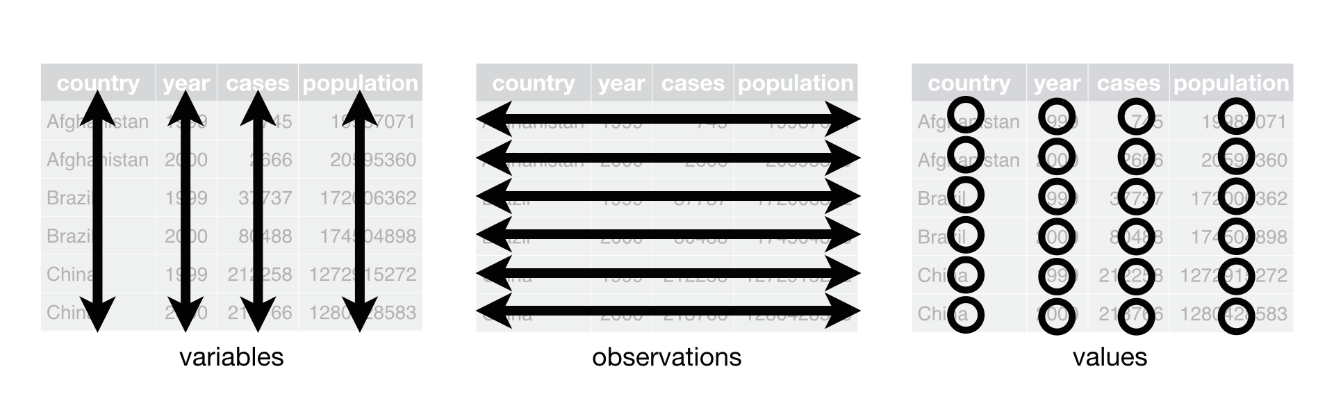
Source: R for Data Science

We have learned the notion of “tidy” data in the second part of the previous module. In short, a dataset is “tidy” when:

Each column is a variable
Each row is an observation
Each cell is a value.

Key `tidyr` functions

In this section, we will learn the following tidyr functions:

gather()
spread()
unite()
separate()
separate_rows()

Please note that, as before, this section is not intended to be an exhaustive documentation and description. For more information, please check out the reference materials listed below.

Make “wide” data longer

gather(tbl, key = "key", value = "value", ..., na.rm = FALSE, ...)

gather() is a function to make “wide” data longer, by “gathering” multiple columns into two columns of key-value pairs. The function takes a tabular data object, such as data.frame or tibble, as its first argument. The second argument, key, defines the name of a new column for key and the third argument, value, defines the name of a new column for value. These two arguments have default values that are, not surprisingly, "key" and "value", respectively.

The following arguments (...) are a selection of columns to be used whose name will be made into values for the key column and whose value will be made into the values of the value column.

Make “long” data wider

spread(tbl, key, value, fill = NA, ...)

spread() is the opposite of gather(). As in gather(), the first argument is a tabular data object. Then, key is an existing column containing the names of new columns, and value is another column containing the values for the new columns.

Example

Let’s take a look at an example illustrating how gather() and spread() work. First, we prepare a data to be used, which is the familiar ispcrime dataset, except we exclude violentCrime and propertyCrime columns using select(). We assign this to ispcrime_2.

ispcrime_2 <- ispcrime %>%
  select(-violentCrime, -propertyCrime) %>%
  as_tibble()

ispcrime_2

## # A tibble: 510 x 10
##     year county  murder  rape robbery aggAssault burglary larcenyTft MVTft
##    <int> <fct>    <int> <int>   <int>      <int>    <int>      <int> <int>
##  1  2011 Adams        0    37      15        166      272       1241    36
##  2  2011 Alexan~      0    14       4        101       92        183    11
##  3  2011 Bond         1     0       0          5       58        147     5
##  4  2011 Boone        0    24       8         27      152        563    14
##  5  2011 Brown        0     1       0          6       14         22     1
##  6  2011 Bureau       0     4       3         35       90        405     8
##  7  2011 Calhoun      0     0       0         13       14         41     1
##  8  2011 Carroll      0     1       0          7       38        165     2
##  9  2011 Cass         0     1       0         11       41         71     3
## 10  2011 Champa~      5   127     208        870     1384       3756   164
## # ... with 500 more rows, and 1 more variable: arson <int>

Now, let’s try gather(). We will name the key column type for the type of crime, and the value column count. Then we will “gather” all 8 crime type columns, from murder to arson. The output is a reshaepd dataset that is 8-times “longer” than the input (4,080 = 510 * 8). The name of each input column is now turned into a value for the type column, and the corresponding crime count is a value for the count column.

ispcrime_2 %>%
  gather(key = "type", value = "count", murder:arson)

## # A tibble: 4,080 x 4
##     year county    type   count
##    <int> <fct>     <chr>  <int>
##  1  2011 Adams     murder     0
##  2  2011 Alexander murder     0
##  3  2011 Bond      murder     1
##  4  2011 Boone     murder     0
##  5  2011 Brown     murder     0
##  6  2011 Bureau    murder     0
##  7  2011 Calhoun   murder     0
##  8  2011 Carroll   murder     0
##  9  2011 Cass      murder     0
## 10  2011 Champaign murder     5
## # ... with 4,070 more rows

Now, to see that spread() is the opposite process, here we show the result of gather()-ing and than spread()-ing the ispcrime_2 object. The final output is in the same shape as the input.

ispcrime_2 %>%
  gather(key = "type", value = "count", murder:arson) %>%
  spread(key = type, value = count)

## # A tibble: 510 x 10
##     year county    aggAssault arson burglary larcenyTft murder MVTft  rape
##    <int> <fct>          <int> <int>    <int>      <int>  <int> <int> <int>
##  1  2011 Adams            166     6      272       1241      0    36    37
##  2  2011 Alexander        101     4       92        183      0    11    14
##  3  2011 Bond               5     1       58        147      1     5     0
##  4  2011 Boone             27     4      152        563      0    14    24
##  5  2011 Brown              6     1       14         22      0     1     1
##  6  2011 Bureau            35     2       90        405      0     8     4
##  7  2011 Calhoun           13     0       14         41      0     1     0
##  8  2011 Carroll            7     1       38        165      0     2     1
##  9  2011 Cass              11     4       41         71      0     3     1
## 10  2011 Champaign        870    28     1384       3756      5   164   127
## # ... with 500 more rows, and 1 more variable: robbery <int>

Unite multiple columns into one

unite(tbl, col, ..., sep = "_", remove = TRUE)

unite() works to combine multiple columns into a single column by concatenating their values. Its first argument is a tabular data object. Then, col is a new column created by “uniting” the following column inputs (...). sep input is a string to be inserted as a seperator between column values when concatenation takes place. The default value for sep is the underscore symbol (_). Finally, remove takes a boolean value for whether removing the original columns or not.

Split a column into many

separate(tbl, col, into, sep = "[^[:alnum:]]+", remove = TRUE, ...)

separate() is the opposite of unite(). As in unite(), the first argument is a tabular data object. Here, col is a column to be split into multiple columns. into is a character vector for separated column names, which may have two or more elements. sep is a separator between values, which could be _, or any other. Finally, remove is a boolean for whether removing the original columns or not.

unite() and sperate() are great for cleaning up date or name variables. One common application is to convert two columns for “last name” and “first name” into a single column for “full name”, or vice versa.

Example

The following example illustrates the use of unite() and separate(). We first prepare a data object for this exercise: we left_join() ispcrime and regions and select() only six columns in the following order: year, region, county, volentCrime, and propertyCrime. This transformed data is assigned to ispcrime_3.

ispcrime_3 <- ispcrime %>%
  left_join(regions) %>%
  select(year, region, county, violentCrime, propertyCrime) %>%
  as_tibble()

## Joining, by = "county"

ispcrime_3

## # A tibble: 510 x 5
##     year region   county    violentCrime propertyCrime
##    <int> <fct>    <fct>            <int>         <int>
##  1  2011 Central  Adams              218          1555
##  2  2011 Southern Alexander          119           290
##  3  2011 Southern Bond                 6           211
##  4  2011 Northern Boone               59           733
##  5  2011 Central  Brown                7            38
##  6  2011 Central  Bureau              42           505
##  7  2011 Southern Calhoun             13            56
##  8  2011 Northern Carroll              8           206
##  9  2011 Central  Cass                12           119
## 10  2011 Central  Champaign         1210          5332
## # ... with 500 more rows

Now, we will try unite() on region and county columns to create a region_county column. Notice that we do not provide any input for sep argument and, accordingly, the default separator, "_", is used to concatenate the two columns.

ispcrime_3 %>%
  unite(col = region_county, region, county)

## # A tibble: 510 x 4
##     year region_county      violentCrime propertyCrime
##    <int> <chr>                     <int>         <int>
##  1  2011 Central_Adams               218          1555
##  2  2011 Southern_Alexander          119           290
##  3  2011 Southern_Bond                 6           211
##  4  2011 Northern_Boone               59           733
##  5  2011 Central_Brown                 7            38
##  6  2011 Central_Bureau               42           505
##  7  2011 Southern_Calhoun             13            56
##  8  2011 Northern_Carroll              8           206
##  9  2011 Central_Cass                 12           119
## 10  2011 Central_Champaign          1210          5332
## # ... with 500 more rows

To see that unite() and separate() are the opposite procedures, we show the result of unite()-ing and separate()-ing the ispcrime_3 data. Note that we have to provide "_" as the sep input to gain back the original input.

ispcrime_3 %>%
  unite(col = region_county, region, county) %>%
  separate(col = region_county, into = c("region", "county"), sep = "_")

## # A tibble: 510 x 5
##     year region   county    violentCrime propertyCrime
##    <int> <chr>    <chr>            <int>         <int>
##  1  2011 Central  Adams              218          1555
##  2  2011 Southern Alexander          119           290
##  3  2011 Southern Bond                 6           211
##  4  2011 Northern Boone               59           733
##  5  2011 Central  Brown                7            38
##  6  2011 Central  Bureau              42           505
##  7  2011 Southern Calhoun             13            56
##  8  2011 Northern Carroll              8           206
##  9  2011 Central  Cass                12           119
## 10  2011 Central  Champaign         1210          5332
## # ... with 500 more rows

Split a row into many

separate_rows(tbl, ..., sep = "[^[:alnum:]]+", ...)

We also have separate_rows(), which is similar to separate(), except the former results in a longer table while the latter results in a wider table.

References

Grolemund, G. & Wickham, H. (2017). R for Data Science.
RStudio. (2017). “Data Import Cheat Sheet”.
RStudio. (2017). “Data Transformation Cheat Sheet”.
Tidyverse. (n.d.). dplyr.tidyverse.org.
Tidyverse. (n.d.). tidyr.tidyverse.org.
Tidyverse. (n.d.). tidyverse.org.

R Workshop: Module 3 (1)

Bobae Kang

March 28, 2018

Links

Data Analysis with R (1): Getting started with tidyverse

Getting Ready

Installing the packages

Importing the packages

Manipulating Your Data

Key dplyr functions

Sort rows by variables

Example

Filter rows with conditions

Example

Select and/or rename variables

Example

Transform and add variables

Example

Merge tables

Example

Aggregate and summarise rows

Example

Group by variables

Example

Chain operations

dplyr in action

Example 1

Example 2

More on dplyr

Tidying Up Your Data

Remember tidy data?

Key tidyr functions

Make “wide” data longer

Make “long” data wider

Example

Unite multiple columns into one

Split a column into many

Example

Split a row into many

More on tidyr

References

Data Analysis with R (1): Getting started with `tidyverse`

`dplyr` in action

More on `dplyr`

Key `tidyr` functions

More on `tidyr`