R Workshop: Module 2 (1)
Bobae Kang
March 22, 2018

This page contains the notes for the first part of R Workshop Module 2: R basics, which is part of the R Workshop series prepared by ICJIA Research Analyst Bobae Kang to enable and encourage ICJIA researchers to take advantage of R, a statistical programming language that is one of the most powerful modern research tools.
Links
Click here to go to the workshop home page.
Click here to go to the workshop Modules page.
Click here to view the accompanying slides for Module 2, Part 1.
Navigate to the other workshop materials:
R Basics (1): Fundamentals of R Programming
Now, let us get started with R for real. Module 2 is design to help you to grasp the fundamental concepts of the R language, which are basic building blocks for using R for data analysis and more!
Key concepts
Here are the key concepts we will be learning in this part:
- Obejcts
- Expressions
- Functions
- Environments
R Objects

Source: Wikimedia Commons
Key object types
In R, anything and everything we use and create is an object. R has various object “types”. Some of the key object types include:
- Vectors (
c()) - Lists (
list()) - Factors (
factor()) - Data frame (
data.frame())
In the following, we will take a deeper look at vectors (a.k.a. atomic vectors) and lists.
“Atomic” vectors
Vector is the most fundamental data type in R, which roughly corresponds to array in other programming languages. Almost everything else in R is built on top of vectors with few exceptions like NULL. In fact, technically, even a single value is a vector of length 1 (this can be verified using the is.vector() function with a single character or number as its input). In that sense, vectors in R are also known as “atomic” vectors.
Basic vector types
Vectors come in different types. Here are the basic vector types:
logical: Boolean values ofTRUEandFALSEdouble: floating-point numbers representing real numbersinteger: integerscomplex: complex numberscharacter: string of alphanumeric letters
Let’s take a look at some examples of these vector types. A vector is created using the c() function. We may think that the “c” means “concatenate”. Note that the class() function returns the vector type for the given object, instead of simply returning vector.
# this is a logical vector
logical_vector <- c(TRUE, FALSE, T, F)

is.logical(logical_vector)
## [1] TRUEclass(logical_vector)## [1] "logical"# this is a double (numeric) vector
double_vector <- c(1, 2, 3)
is.double(double_vector)## [1] TRUEclass(double_vector)## [1] "numeric"# this is an integer (numeric) vector
integer_vector <- c(1L, 2L ,3L)
is.integer(integer_vector)## [1] TRUEclass(integer_vector)## [1] "integer"# this is a character vector
character_vector <- c("a", "b", "c")
is.character(character_vector)## [1] TRUEclass(character_vector)## [1] "character"# an object with a single element is also a vector!
x <- 1
y <- "Am I a vector?"
is.vector(x)## [1] TRUEis.vector(y)## [1] TRUEAccessing vector elements
A vector often comes as a series of multiple values or elements–this is probably why it is called a “vector”, like a mathematical vector.
To access a particular element in a vecgtor, we can use the index of an element with []:
fruits <- c("apple", "banana", "clementine")
first_fruit <- fruits[1]

print(first_fruit)
## [1] "apple"second_fruit <- fruits[2]
print(second_fruit)## [1] "banana"We can also assign a new value to the accessed vector element:
# giving a new value to an existing element
fruits[1] <- "apricot"

print(fruits)
## [1] "apricot" "banana" "clementine"Or create a new element:
# creating a new element
fruits[4] <- "dried mango"

fruits
## [1] "apricot" "banana" "clementine" "dried mango"Multiple elements can be accessed in two ways. First, we can use a vector of indices:
first_and_third_fruits <- fruits[c(1, 3)]

print(first_and_third_fruits)
## [1] "apricot" "clementine"Second, we can use the colon operator for a sequence (we will come back to the colon operator):
first_thru_third_fruits <- fruits[1:3]

print(first_thru_third_fruits)
## [1] "apricot" "banana" "clementine"Vector elements can be accessed conditionally as well:
my_vector <- c(1, 2, 3, 4, 5)

# print only elements less than 3
print(my_vector[my_vector < 3])
## [1] 1 2# assign 0 to such elements
my_vector[my_vector < 3] <- 0
print(my_vector)## [1] 0 0 3 4 5Lists
An R vector cannot consist of elements of different vector types. Considering that a single element is in fact a vector of length 1, we can see how such an idea is a simple impossibility.
In contrast, an R list, created by list() function, can contain elements of different types. A list is, in fact, a list of vectors:
my_list <- list("abc", 125, FALSE, c("Hello", "World"))

print(my_list)
## [[1]]
## [1] "abc"
##
## [[2]]
## [1] 125
##
## [[3]]
## [1] FALSE
##
## [[4]]
## [1] "Hello" "World"Note that an element of a list can be a vector of length greater than 1. In fact, a list can have a nested structure, where an element of a list is also a list itself.
Naming list elements
names(my_list) <- c("character", "numeric", "logical", "character vector")

my_list
## $character
## [1] "abc"
##
## $numeric
## [1] 125
##
## $logical
## [1] FALSE
##
## $`character vector`
## [1] "Hello" "World"Accessing list elements
Elements in a list can be accessed using their indices or names:
# using index (this returns a list element, NOT the actual content)
my_list[4]
## $`character vector`
## [1] "Hello" "World"# using name (this returns the content itself)
my_list$`character vector`## [1] "Hello" "World"In order to access the content of a list element using the index approach, we must use [[]] instead:
my_list[[1]]## [1] "abc"# the result is the same with accessing an element using name
identical(my_list[[1]], my_list$character)## [1] TRUE# in contrast:
identical(my_list[1], my_list$character)## [1] FALSELists to vector
A list can be “unlisted”, i.e., converted into a vector. This is achieved by the unlist() function:
new_list <- list(1:5)
to_vector <- unlist(new_list)

# this is a list
print(new_list)
## [[1]]
## [1] 1 2 3 4 5# this is a vector
print(to_vector)## [1] 1 2 3 4 5R Expressions
Source: clker.com
What are expressions
A program can be seen as a collection of expressions, which are executable pieces of code. In R, an expression consists of the following:
- objects
- operators
- control structures, and
- functions
We have already seen objects. We will now take a closer look at the rest of them.
Operators
Operators are used to manipulate objects in R. They are like functions but used without the parentheses, (), required to invoke a function. Let use take a look at some of the operators in R:
- Arithmetic operators
- Logical operators
- Relational operators
- Assignment operators
- Miscellaneous operators
- Others
- User-defined operators
- From third-party pacakges
Arithmetic operators
The following table lists operators for basic arithmetics:
| Operator | Description | Example |
|---|---|---|
+ |
Addition | 1 + 1 (returns 2) |
- |
Substraction | 3 - 2 (returns 1) |
* |
Multiplication | 3 * 4 (returns 12) |
/ |
Division | 5 / 2 (returns 2.5) |
^ or ** |
Exponentiation | 2**4 (returns 16) |
%% |
Modulus | 5 %% 2 (returns 1) |
%/% |
Integer division | 5 %/% 2 (returns 2) |
Logical operators
The following table lists logical operators for booelan values:
| Operator | Description | Example |
|---|---|---|
& |
Element-wise logical AND | c(TRUE, TRUE) & c(TRUE, FALSE)returns TRUE FALSE |
| | | Element-wise logical OR | c(TRUE, FALSE) | c(FALSE, FALSE)returns TRUE FALSE |
! |
Logical NOT | !c(TRUE, FALSE)returns TRUE |
&& |
Logical AND (considers the first element only) |
c(TRUE, TRUE) && c(FALSE, TRUE)returns FALSE |
| || | Logical OR (considers the first element only) |
c(TRUE, TRUE) || c(FALSE, TRUE)returns TRUE |
Relational operators
The following table lists relational operators used to compare the values of two objects:
| Operator | Description | Example |
|---|---|---|
> |
Greater than | 3 > 1 returns TRUE |
< |
Less than | 3 < 1 returns FALSE |
== |
Equal to | 2 == 2 returns TRUE |
>= |
Greater than or equal to | 3 >= 4 returns FALSE |
<= |
Less than or equal to | 4 <= 4 returns TRUE |
!= |
Not equal to | 2 != 3 returns TRUE |
Assignment operators
The following table lists assignment operators used to create/modify variables:
| Operator | Description | Example |
|---|---|---|
<- or = |
Left assignment | a <- "Hello" assigns "Hello" to the object a |
-> |
Right assignment | The use of -> is mostly discouraged |
<<- |
Left scoping assignment | Search for the variable in the parent environments takes place before assignment |
->> |
Right scoping assignment | Ditto |
Miscellaneous operators
The following table lists some miscellaneous operators:
| Operator | Description | Example |
|---|---|---|
: |
Colon operator to generate sequences | 1:10 generates a vector of integer sequence from 1 to 10 |
? |
Help function to see documentation | ?my_function is equivalent to help(my_function) |
$ |
List subset | my_list$a will access the subset a in the list |
%in% |
“In” operator | 1 %in% c(1,2,3) returns TRUE |
%*% |
Matrix multiplication |
Other operators
In practice, using R operators is no different from a function call. Accordingly, it is also possible to define new operators. In fact, some third party packages offer custom operators. One such example is the “pipe” operator (%>%) from magrittr package, which is also available through dplyr pacakge.
Flow control
By default, R runs statements in a sequential manner, from top to bottom. There are however ways to break from this using contronl structures. Here we call it “flow control”.
In the following, we will take a look at two basic flow control methods: conditionals and loops.
Conditionals
Using conditionals means creating a desired “flow” of evaluating statements based on certain conditions: i.e. if A, then B.
R offers if statement to acheieve this. The basic if statement structure is given as follows:
if ( condition ) { expression }
Let’s try an example:
a <- TRUE

if (a) {
  print("Hello World!")
}
## [1] "Hello World!"Here, the variable a is a condition to be tested. If the value of the condition is boolean TRUE, than the statements between curly braces {} are executed. If the condition value is FALSE, R jumps ahead the statemetns between {}.
Multiple conditions
It is possible to create more elaborate flow control structures. R provides else statement for the statements to run only if the preceding if condition is FALSE. Then, we can chain multiple if-elses to incorporate multiple conditions.
The following code block presents an example of chained if-else statement with three conditions: (1) a is greater than b, (2) a is not greater but is less than b, (3) a is neither greater or less than b. R evaluates these conditions in a sequential manner, and when the condition evaluates as TRUE, executes the relevant statements.
a <- 1
b <- 2
if (a > b) {
print("a is larger than b.")
} else if (a < b) {
print("a is smaller than b.")
} else {
print("a and b are equal!")
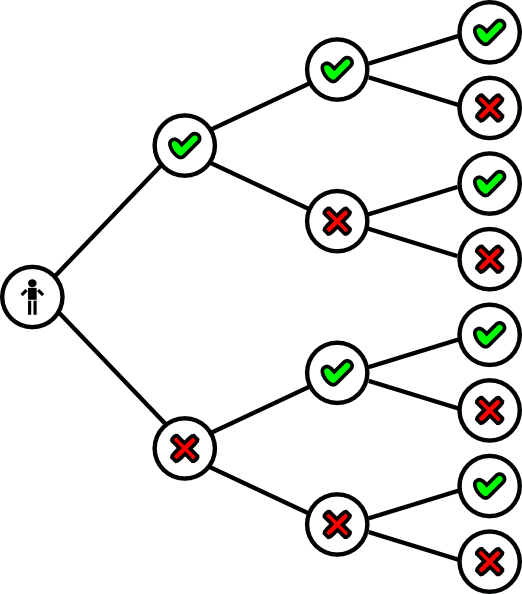
}## [1] "a is smaller than b."ifelse function
ifelse(test_expression, true_value, false_value)R also offers ifelse function, which is to try the condition for each element of a multi-element object. That is, ifelse() is an element-wise if-else conditional. Here, the given condition (test_expression) is tested for each and every element of a vector and the output is a vector of the same length with relevant values.
In the following example, ifelse will return a vector of 4, which equals to the length of input vector a, and the each element of the output vector is the result of testing whether the input element is less than 3.
a <- c(1,2,3,4)
ifelse(a < 3, "Less than 3", "Not less than 3")
## [1] "Less than 3" "Less than 3" "Not less than 3" "Not less than 3"Loops
R offers looping statements for tasks that involve some repetitions. Here we will take a look at two commonly used looping methods: while and for.
whileloops
while ( condition ) {
  expression
}forloops
for (element in iterable_object) {
  expression
}
while loop
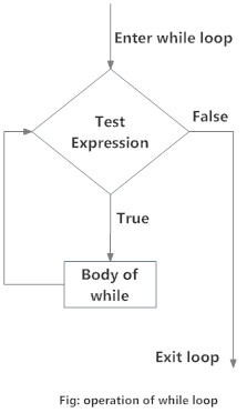
Source: DataMentor
A while loop consists of a condition and a group of statments (expression) to be executed.
while (condition) {
  expression
}
while statement goes through the following steps:
- If the given
conditionis satisfied (i.e. evaluates asTRUE), then the followingexpressionis executed. - Once the
expressionis executed, theconditionis re-evaluated. - The
expressionis repetitively executed as long as theconditionis satisfied.
This means that, if the condition is always TRUE, we will be stuck in an infinite loop!
The folloing example uses while statement to print a number from 0 to 4. Because we add 1 to count at each loop, we can be rest assured that the condition will return FALSE at one point, and the loop will terminate.
count <- 0

while (count < 5) {
  print(count)
  count = count + 1  # increase count by 1 at each iteration
}
## [1] 0
## [1] 1
## [1] 2
## [1] 3
## [1] 4for loop
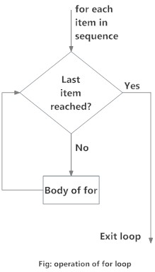
Source: DataMentor
A for loop is similar to while loop, except that it takes an iterable object (vector or list) rather than a condition.
for (element in iterable_object) {
  expression
}
Intead of checking for a condition, for loop iterates over all elements of the given object in order. The loop terminates when we reach the final element of the iterable object. At each step of iteration, we can use the given element for the expression if appropriate.
Let’s try couple examples.
In the first example, we directly iterate over the elements of fruits vector. At each step, the value of fruit changes and made available between the curly braces as a variable. In this example, the paste() function is used to concatenate multiple character strings into one.
fruits <- c("apple", "banana", "clementine")

# iterate over elements directly
for (fruit in fruits) {
  print(paste("I love ", fruit, "!", sep=""))
}
## [1] "I love apple!"
## [1] "I love banana!"
## [1] "I love clementine!"In the second example, we indirectly iterate over the flavors vector using indices.
flavors <- c("chocolate", "vanilla", "cookie dough")

# iterate over elements indirectly
for (i in 1:length(flavors)) {
  flavor <- flavors[i]
  print(paste("Do you want some", flavor, "ice cream?"))
}
## [1] "Do you want some chocolate ice cream?"
## [1] "Do you want some vanilla ice cream?"
## [1] "Do you want some cookie dough ice cream?"break statement
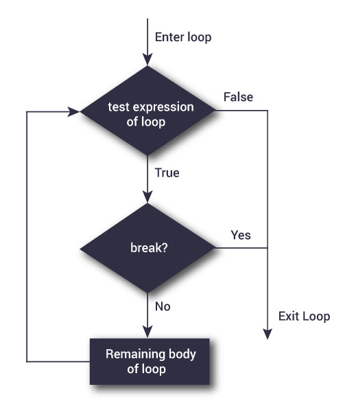
Source: DataMentor
By combining conditionals and loops, we can generate a more complex flow control structure. Here we introduce two additional statements, break and next, which support creating advanced control structure.
# with for loop
for (element in iterable_object) {
  if (break_condition) {
    break
  }
  expression
}

# with while loop
while (loop_condition) {
  if (break_condition) {
    break
  }
  expression
}
break statment is used to “break out”of the loop when certain condition is met.
next statement
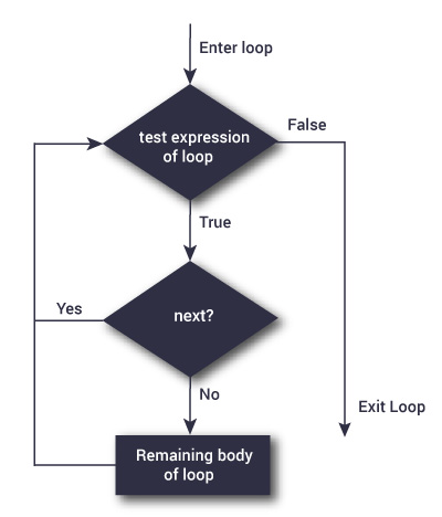
Source: DataMentor
# with for loop
for (element in iterable_object) {
  if (next_condition) {
    next
  }
  expression
}

# with while loop
while (loop_condition) {
  if (next_condition) {
    next
  }
  expression
}
next statement can be used to skip a step in a loop when a certain condition is met.
R Functions

Source: Wikimedia Commons
What are functions
In R, functions are special objects that are “call-able”. In other words, a function can be called or invoked by following (). Meanwhile, a function can be manipulated just in the same way as any other object.
There are three elements of a function (or function closure):
- an argument list (a.k.a. parameters; optional)
- body
- function environment
Why use functions
A key function of a function (pun intended :)) is to encapsulate repeated operations so that we can:
- Simplify code (clearner and more concise)
- Avoid unintended bugs/errors
- Enhance reproducibility
In other words, if you find yourself copying and pasting the same code chunk over and over, you should wrap it into a function.
Creating a new function
# creating a new function
name <- function(arg1, arg2) {

  # body exist in a local environment
  body expression1
  body expression2
  body expression3

}
Just as we assign some values to a symbol (or a variable) to create an object, we assign a function() {} to a symbol to create a function. We put a number of arguments, or parameters, into the (), and a set of operations in {}, where the parameters can be used to represent actual inputs.
It must be noted that the expressions inside {} are living in a “function environment” that is “closed” off of the global environment. We will talk more about environments later. For now, we should only remember the following key points:
- Objects created in a function environment are not accessible from its parent environment
- Objects existing in the parent environment are accessible from the the function environment
- Each function call creates a separate environment (or an instance of the function environment)
Now, let’s take a look at some examples to explore how we can create a function.
A custom function for adding two numbers
# example: a custom function for adding two numbers
add_nums <- function(num1, num2) {
  return(num1 + num2)
}

add_output <- add_nums(3, 5) # assign the function output to a variable

print(add_output)
## [1] 8In this example, we create a function add_nums, which takes two numbers as arguments and returns the sum of the two numbers. The output value that the function returns can be assigned to create an object.
A function without arguments
# example: a custom function without arguments
print_hello_world <- function() {
  print("Hello world")
}

print_hello_world()
## [1] "Hello world"Here, we create a function print_hello_world, which has no argument input. That is, we are not required to have arguments to create a function. In fact, the function also has no real output–it just prints a phrase. Calling the function will print the phrase.
A function with arguments having default values
add_nums_2 <- function(num1, num2 = 5) {
  num1 + num2
}

add_nums_2(3) # call a function using the default value for num2
## [1] 8A function can be given default values to its arguments. If the argument value is not given when the function is called, the default value is used for that argument. It is a good practice to make default values something that are expected to be used most often when calling the function.
R Environments
Source: Hadley Wickham, 2017, Advanced R
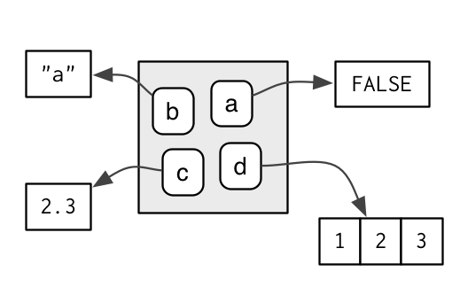
What are environments
Environment is a tricky concept to grasp. Simply put, an environment is a place to store variables. That is, all variables (as bindings of symbols and objects) exist in a specific environment. More precisely, objects live in memory outside all environment; it is the symbols and the associations of the symbols (variable names) and objects to which the symbols point/refer that an environment contains.
As we will see shortly, environments can have a nested structure.
Nesting of environments
There are two simple rules to know about the nesting of environments:
- Variables in a parent environment are accessible in a child environment
- Variables in a child environment are NOT accessible in a parent environment
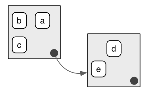
Source: Hadley Wickham, 2017, Advanced R
In this picture, the box on the left represents a parent environment and the box on the right is a child environment. Variables a, b, and c are stored in the parent environment while d and e are in the child environment. According to the two basic rules about environments, accessing variables d and e from the parent environment is not possible but, a, b, and c are still accessible from the child environment.
The global environment
There is something called “global environment” in R, which deserves our special attention. In short, the global environment serves as the interactive workspace for the given R session. When we create new variables using the console, they will live in the global environment.
The immediate parent of the global environment is the environment of the package that is imported last. This is how all the datasets and functions from the package, as well as other pacakges imported prior to it, are made available in the global environment.
In R, an environment is like a function, and the global environment can be accessed using globalenv(), which works like a named list as shown in the folloing code chunk:
some_variable <- 1 # a variable in the global environment
global_env <-globalenv() # the environment itself can be assigned to a variable

# the following two are identical
identical(some_variable, global_env$some_variable)
## [1] TRUELocal environments
If there is the global environment, there are local environments as well. Local environments are created in two ways:
* any function calls
* `new.env()`
A local environment can be used to protect the global environment from arbitrarily created variables.
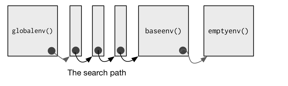
Lexical scoping
Searching for an object in R follows the lexical scoping rules.
- First, R looks for the object in the current environment
- If the object is not found in the current environment, R moves up to its parent environment.
- The process is repeated until the object is found or the outermost environment (
emptyenv()) is reached.
Source: Hadley Wickham, 2017, Advanced R
References
- DataMentor. (n.d.). R Tutorials
- R Core Team. (2017). “An Introduction to R”.
- R Core Team. (2017). “R Language Definition”.
- Wickham, H. (2017). Advanced R.